How it works
Theory Demos
Each demo takes one result from ML theory and builds the smallest numerical case where you can watch it happen. Below is the idea at the heart of each of the five scripts, the few lines of numpy that carry it, the figures they produce, the tests that hold the code to the math, and how the browser demos on the project page port it all to JavaScript.
- Learning theory
- Probability & statistics
- Plain numpy
- Privacy & robustness
Every demo, the same recipe
- Claimone theorem or formula from the literature
- Buildthe smallest setup where it shows: 12 points, 2-D data
- Measuresimulate many times, print beside the formula
- Plotsave one figure to
out/ - Testpytest asserts the claim still holds
The ideas
- 01More parameters can mean less error
- 02High dimensions are mostly empty corners
- 03A perfect diffusion model only copies
- 04Lie on purpose, then undo it on average
- 05Guarantees instead of attacks
- 06Tests that check the theorems
- 07The same maths, in your browser
- →Browser vs Python
- →Limits
- →Reproduce
- →References
- →Read further
More parameters can mean less error
Double descent with random Fourier features
Twelve noisy samples of sin(2πx) are fit with p random cosine features. Classical intuition says error should keep rising once the model can fit the noise. Instead it spikes at p = n = 12 and then falls again. The whole effect lives in which solution the fit returns once there are more features than points (Belkin, Hsu, Ma & Mandal, 2019).
def features(x, w, b):
    return np.sqrt(2.0 / len(w)) * np.cos(np.outer(x, w) + b)


def fit(F, y, ridge=0.0):
    """Min-norm least squares (ridge=0) or ridge regression, via the dual form
    when p > n (cheaper and identical)."""
    n, p = F.shape
    if ridge == 0.0:
        return np.linalg.pinv(F, rcond=1e-13) @ y
    if p > n:
        return F.T @ np.linalg.solve(F @ F.T + ridge * np.eye(n), y)
return np.linalg.solve(F.T @ F + ridge * np.eye(p), F.T @ y)- Each feature is
cos(w·x + b)with a random frequency and phase. The √(2/p) scaling keeps the model's output on the same scale as p grows. - The pseudo-inverse gives ordinary least squares when p < n and, when p ≥ n, the interpolant with the smallest weight norm. That is also where gradient descent started from zero ends up.
- With a ridge penalty and p > n, the code solves an n × n system instead of a p × p one. Same answer, far cheaper at p = 2000.
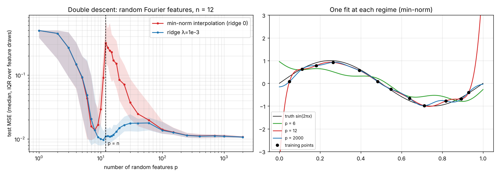
Median over 100 feature draws: test MSE 0.0138 at the best p = 8, 0.3165 at p = 12 (23× worse), 0.0108 at p = 2000. A ridge of 1e-3 keeps the worst value near p = n at 0.0165.
Whether the second descent ends below the first minimum depends on the noise level and the feature bandwidth. Here it does (0.0108 against 0.0138), but that isn't a universal law. The noise slider in the browser demo lets you see this move.
High dimensions are mostly empty corners
Near-orthogonality, thin shells and packing
Three facts that surprise people the first time, each checked by sampling. The basic tool is a uniformly random direction: draw a Gaussian vector and divide by its length. The cosine between two such directions is then just a dot product, and its spread should be exactly 1/√d.
def random_unit(n, d, rng):
    v = rng.standard_normal((n, d))
    return v / np.linalg.norm(v, axis=1, keepdims=True)


def cosine_samples(d, n_pairs=20000, seed=0):
    """Cosines between n_pairs independent pairs of random unit vectors."""
    rng = np.random.default_rng(seed)
    out = np.empty(n_pairs)
    batch = max(1, min(n_pairs, 2_000_000 // d))
    for s in range(0, n_pairs, batch):
        m = min(batch, n_pairs - s)
        u, v = random_unit(m, d, rng), random_unit(m, d, rng)
        out[s:s + m] = (u * v).sum(axis=1)
return out- A standard Gaussian looks the same in every direction, so normalising it gives a direction drawn uniformly from the sphere.
- Batches are sized so each holds about two million numbers, which keeps memory flat whether d is 2 or 10,000.
- Row-wise dot products of unit vectors are the cosines. Measured spreads: 0.3175, 0.1010, 0.0319, 0.0101 for d = 10 to 10,000, against 1/√d = 0.3162 … 0.0100.
How many directions fit with every pairwise |cos| below 0.1? Only d can be exactly orthogonal, but near-orthogonal sets grow exponentially. The squared cosine of two random directions follows a known Beta law, so the chance that one pair breaks the rule has an exact formula and no simulation is needed:
def pair_violation_prob(d, thresh=0.1):
    """Exact P(|cos| >= thresh) for two random unit vectors in R^d:
    cos^2 ~ Beta(1/2, (d-1)/2)."""
    from scipy import stats
return float(stats.beta.sf(thresh**2, 0.5, (d - 1) / 2))- cos² ~ Beta(½, (d−1)/2), so |cos| ≥ 0.1 is the event cos² ≥ 0.01.
- The survival function gives that tail probability pd. A birthday argument turns it into a set size of about √(2 ln 2 / pd): about 30 vectors at d = 1,000, about 77,000 at d = 4,000 and a million at d = 5,000.
A search does better than a random set. The greedy search draws 20,000 random directions and keeps each one that is within |cos| < 0.1 of every direction kept so far. At d = 800 it keeps 972, already more than d. The growth is exponential, but it starts late.
The third fact needs no sampling at all: the share of a ball's volume within ε of its surface is 1 − (1 − ε)d. At d = 100, 99.997% of the volume is in the outer 10% of the radius. The script checks the formula by Monte Carlo for d ≤ 8, where rejection sampling from the cube still works.
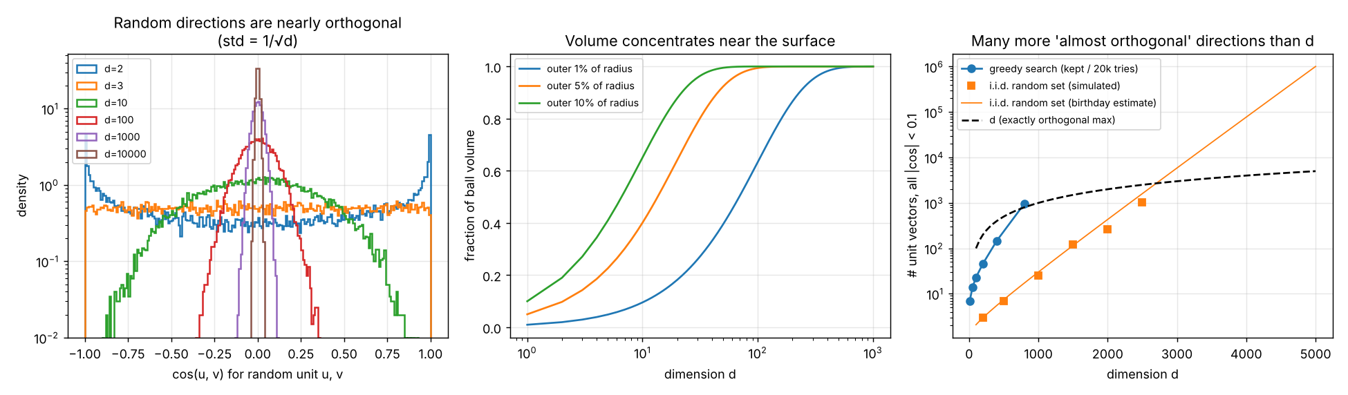
high_dim.py: cosine spread against 1/√d, the share of volume near the surface, and how many near-orthogonal vectors fit.A perfect diffusion model only copies
The exact score of the training set
A diffusion model learns the score, the gradient of log-density, of noised data. For a finite training set the noised distribution is a mixture of Gaussians centred on the training points, and its score has a closed form. So the demo can skip training and ask: what does the ideal model generate? A sampler with that exact score reproduces the training points. A perfect model memorises, which is the effect behind training-data extraction from real diffusion models (Carlini et al., 2023).
∇ log pσ(x) = Σi wi(x) (xi − x) / σ², w = softmax(−|x − xi|² / 2σ²)
def exact_score(x, sigma, train):
    """Score of (1/N) sum_i N(x_i, sigma^2 I) at points x (n, 2)."""
    d2 = ((x[:, None, :] - train[None, :, :]) ** 2).sum(-1)       # (n, N)
    logits = -d2 / (2 * sigma**2)
    w = np.exp(logits - logits.max(axis=1, keepdims=True))
    w /= w.sum(axis=1, keepdims=True)
return (w @ train - x) / sigma**2- Squared distance from every sample to every training point, by broadcasting: shape (samples, training points).
- A softmax over training points, with the max subtracted first so
expnever overflows when σ is as small as 0.01. - The score points from x toward a weighted average of training points. As σ shrinks, the weights pick out the single nearest point.
def reverse_sample(score_fn, n, rng, n_steps=500, train=None):
    """x_{k+1} = x_k + (s_k^2 - s_{k+1}^2) score(x_k, s_k) + sqrt(s_k^2 - s_{k+1}^2) z.
    The last step uses no noise (Tweedie-style denoise)."""
    sig = sigma_schedule(n_steps)
    x = SIGMA_MAX * rng.standard_normal((n, 2))
    for k in range(n_steps):
        dv = sig[k] ** 2 - sig[k + 1] ** 2
        x = x + dv * score_fn(x, sig[k], train)
        if k < n_steps - 1:
            x = x + np.sqrt(dv) * rng.standard_normal(x.shape)
return x- Start from pure noise at σ = 3 and walk the noise level down a geometric schedule to 0.01.
- Each step moves along the score by the drop in variance. Any score function plugs in here: exact, blurred, or the trained MLP.
- Fresh noise is added on every step but the last, which is a pure denoising step.
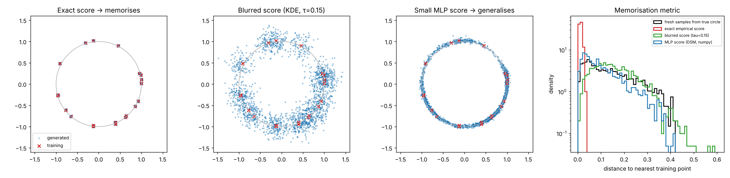
With the exact score, 99.0% of 2,000 samples land within 0.03 of a training point. The MLP trained by denoising score matching gives 17.5%, close to the 11.3% of fresh samples from the true circle.
Two imperfect scores generalise instead. The blurred score uses the exact score at a larger noise level, √(σ² + τ²), which makes it a kernel density estimate with bandwidth τ. The MLP has 64-unit layers, is trained for 4,000 Adam steps in numpy, and its limited capacity spreads mass along the circle. Full numbers, 20 training points and 2,000 samples per row:
| source | median distance to nearest training point | copies | median |r − 1| |
|---|---|---|---|
| Fresh samples from the true circle | 0.1235 | 11.3% | 0.0136 |
| Exact empirical score | 0.0115 | 99.0% | 0.0121 |
| Blurred score (τ = 0.15) | 0.1482 | 3.1% | 0.1035 |
| MLP score | 0.0845 | 17.5% | 0.0154 |
The MLP's samples stay on the circle and are mostly not copies. The blur generalises by smearing samples off the circle, which isn't the same as learning the shape. A bigger network trained much longer would drift back toward the memorising exact score.
Lie on purpose, then undo it on average
Randomized response and local differential privacy
Warner's 1965 survey trick: each person secretly answers either the real question (with probability p) or its opposite. No single “yes” reveals anything for sure, but the mixing is known, so the population rate can be solved for. Each answer is ε-locally differentially private with ε = ln(p / (1 − p)).
P(yes) = λ = pπ + (1 − p)(1 − π) ⇒ π̂ = (λ̂ − (1 − p)) / (2p − 1)
def respond(truth: np.ndarray, p: float, rng) -> np.ndarray:
    """Randomized answers (bool) for true memberships `truth` (bool)."""
    asks_direct = rng.random(truth.shape) < p
    return np.where(asks_direct, truth, ~truth)


def estimate(n_yes, n, p):
    """Unbiased Warner estimator and its plug-in standard error."""
    lam = n_yes / n
    pi_hat = (lam - (1 - p)) / (2 * p - 1)
    se = np.sqrt(lam * (1 - lam) / n) / abs(2 * p - 1)
return pi_hat, se- The respondent's side: a private coin decides whether they answer truthfully or answer the complement question. The analyst sees only the result.
- The formula above, inverted. It is unbiased because λ̂ is, and the map from λ to π is linear.
- Dividing by |2p − 1| is the price of privacy. As p nears ½ the noise blows up: at p = 0.6 you need 29.6× as many respondents as an honest survey.
def confidence_interval(n_yes, n, p, conf=0.95):
    """Exact (Clopper-Pearson) interval for lambda = P(yes), mapped through the
    linear Warner transform and clipped to [0, 1].  Conservative but valid."""
    a = 1 - conf
    lo = stats.beta.ppf(a / 2, n_yes, n - n_yes + 1) if n_yes > 0 else 0.0
    hi = stats.beta.ppf(1 - a / 2, n_yes + 1, n - n_yes) if n_yes < n else 1.0
    ends = sorted(((lo - (1 - p)) / (2 * p - 1), (hi - (1 - p)) / (2 * p - 1)))
return max(0.0, ends[0]), min(1.0, ends[1])- An exact binomial interval for the raw yes-rate λ, written with Beta quantiles, with the edge cases of all-no or all-yes handled.
- Because π is a linear function of λ, the interval's ends map straight across. Sorting covers p < ½, where the map flips direction.
- Clipping to [0, 1] keeps the interval meaningful even when the point estimate falls outside it by chance.
The price is precision: you need more respondents. Simulated with a true rate of 0.3:
| design | ε | spread of estimate (n = 1,000) | respondents needed vs honest survey |
|---|---|---|---|
| p = 0.6 | 0.41 | 0.081 | 29.6× |
| p = 0.75 | 1.10 | 0.031 | 4.6× |
| p = 0.9 | 2.20 | 0.019 | 1.7× |
| honest answers | — | 0.0145 | 1× |
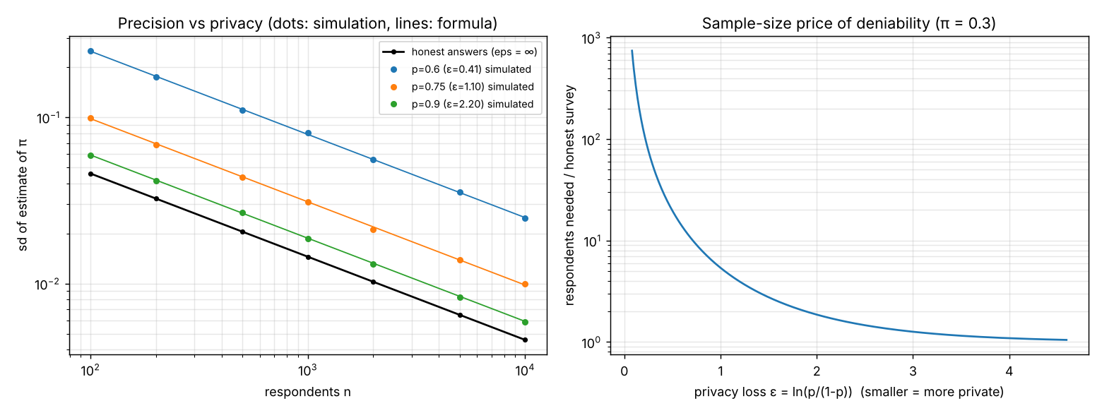
randomized_response.py. Simulated estimates match the theoretical variance; stronger privacy (smaller ε) costs many more respondents.The same functions back a command-line tool for real surveys, and the browser demo has the same analysis built in. On the 800-answer example poll it estimates 0.305 with exact interval [0.237, 0.375]; the true fraction in that file is 0.283.
python randomized_response.py poll out/example_poll.csv --p 0.75 --column answer
Guarantees instead of attacks
Lipschitz margins and randomized smoothing
An attack can show a classifier is fragile; it can never show it is safe. A certificate can. If the score f changes by at most L per unit of input distance, then no change smaller than |f(x)| / L can flip its sign. The demo builds this two ways on the two-moons dataset, with networks written in numpy: a wiggly unconstrained net, and one with every weight matrix projected to spectral norm ≤ 1, so L ≤ 1. Both are also attacked with PGD.
    def project_spectral(self, max_norm=1.0):
        for W in self.W:
            s = np.linalg.norm(W, 2)
            if s > max_norm:
                W /= s / max_norm

    def lipschitz_bound(self):
        """Valid global l2 Lipschitz constant (ReLU is 1-Lipschitz)."""
return float(np.prod([np.linalg.norm(W, 2) for W in self.W]))- Called after every Adam step for the constrained net: any weight matrix whose largest singular value exceeds 1 is scaled back to 1, in place.
- Each layer stretches distances by at most its spectral norm and ReLU never stretches them, so the product is a valid bound. It is 1 for the constrained net and about 2,000 for the unconstrained “wiggly” one.
The certified radius is then just np.abs(net(X)) / net.lipschitz_bound(). For the wiggly net that radius is useless, so the demo certifies it a second way: randomized smoothing (Cohen, Rosenfeld & Kolter, 2019) classifies by majority vote over Gaussian-noised copies of the input, and the margin of that vote gives a radius.
def smoothed_certify(net, X, sigma, n0=100, n=10000, alpha=0.001, seed=0, chunk=2000):
    """Cohen et al. CERTIFY for binary h = sign(f).  Returns (prediction in
    {-1, 0 (abstain), +1}, certified radius)."""
    rng = np.random.default_rng(seed)
    preds, radii = np.zeros(len(X)), np.zeros(len(X))
    for i, x in enumerate(X):
        sel = np.sign(net(x + sigma * rng.standard_normal((n0, 2))))
        cA = 1.0 if (sel > 0).sum() >= (sel < 0).sum() else -1.0
        k = 0
        for s in range(0, n, chunk):
            m = min(chunk, n - s)
            k += int((np.sign(net(x + sigma * rng.standard_normal((m, 2)))) == cA).sum())
        pA_low = stats.beta.ppf(alpha, k, n - k + 1) if k > 0 else 0.0  # one-sided CP
        if pA_low > 0.5:
            preds[i], radii[i] = cA, sigma * stats.norm.ppf(pA_low)
return preds, radii- A first, small batch of 100 noisy votes only picks the likely winning class. Using separate samples to choose and to certify keeps the statistics honest.
- Then 10,000 fresh noisy copies count how often that class wins, in chunks to bound memory.
- A one-sided Clopper–Pearson lower bound on the win rate, so the certificate holds with probability at least 1 − α = 99.9%.
- If the lower bound beats ½, the radius is σΦ⁻¹(pA); otherwise the point gets radius 0 and the prediction abstains.
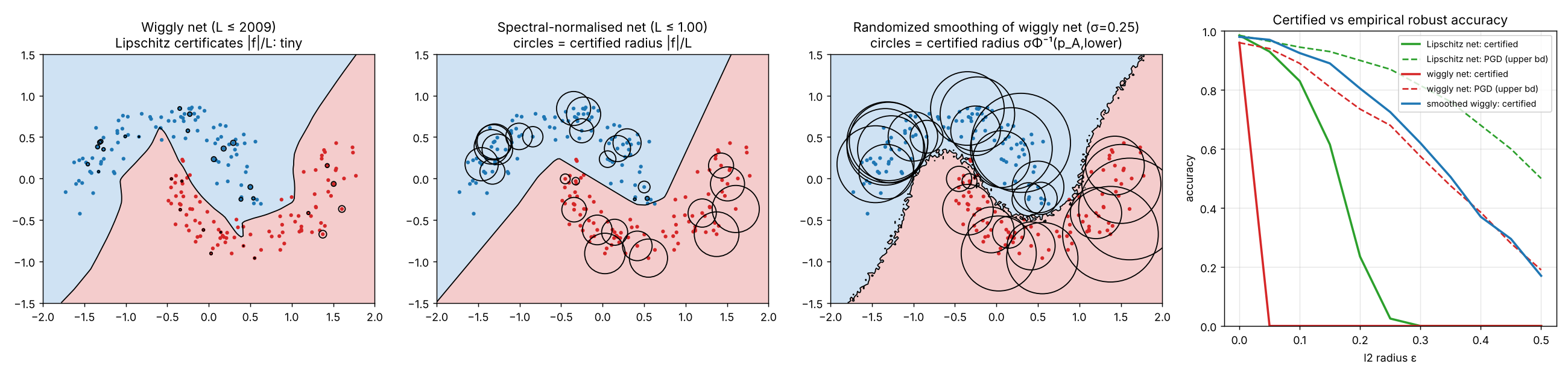
| radius | Lipschitz net, certified | Lipschitz net, PGD | wiggly net, certified | wiggly net, PGD | smoothed, certified |
|---|---|---|---|---|---|
| 0.0 | 0.985 | 0.985 | 0.960 | 0.960 | 0.980 |
| 0.1 | 0.830 | 0.945 | 0.000 | 0.890 | 0.925 |
| 0.2 | 0.235 | 0.900 | 0.000 | 0.735 | 0.805 |
| 0.3 | 0.000 | 0.815 | 0.000 | 0.575 | 0.620 |
Certified accuracy on 200 test points, σ = 0.25 for smoothing. PGD found 0 violations inside the Lipschitz net's 197 certified radii, as it must. The wiggly net is fairly robust in practice, but its Lipschitz bound of about 2,000 certifies nothing. Smoothing turns the same network into a certifiable classifier. Strictly, it certifies the smoothed classifier, not the original network.
Tests that check the theorems
18 pytest cases that hold the code to the math
A demo of a theorem is only convincing if the code is right, so each claim is also a test: the cosine spread matches 1/√d, the double-descent peak exists and ridge removes it, the Warner estimator is unbiased, the exact score matches finite differences. The strongest ones try to break a guarantee and must fail.
def test_lipschitz_bound_is_valid(models):
    _, _, lip = models
    rng = np.random.default_rng(0)
    a, b = rng.uniform(-2, 2, (5000, 2)), rng.uniform(-2, 2, (5000, 2))
    ratio = np.abs(lip(a) - lip(b)) / np.linalg.norm(a - b, axis=1)
    assert ratio.max() <= lip.lipschitz_bound() + 1e-9 <= 1 + 1e-9


def test_certified_radius_never_violated_by_attack(models):
    (_, _, Xte, yte), wiggly, lip = models
    for net in (lip, wiggly):
        correct = yte * net(Xte) > 0
        rad = cr.lipschitz_radius(net, Xte)
        m, xadv = cr.pgd_attack(net, Xte, yte, 0.999 * rad, steps=40, restarts=2)
        assert np.all(m[correct] > 0)
assert np.all(np.linalg.norm(xadv - Xte, axis=1) <= rad + 1e-9)- Measure the slope of the trained net between 5,000 random pairs of points. None may exceed the claimed bound, and the bound itself must be at most 1.
- Attack every test point with projected gradient descent, restricted to just inside its certified radius.
- The attack must never flip a correct prediction, and must really have stayed inside the radius. In the full run, PGD found 0 violations across 197 certified points.
The same maths, in your browser
Plain JavaScript ports of the five scripts
The project page runs all five experiments live, with no server. web/lib.js holds the maths, one function per Python function, and names the function it ports. web/worker.js runs anything slow in a Web Worker so the page never freezes, and web/demos.js draws the plots on canvas. There are no libraries: the SVD, the Beta and normal quantiles that scipy provides, and the small neural network are written out by hand.
The setups are the scripts' own: 12 points, cosine features with frequency scale 15 and a 500-point test grid for double descent; 20 points on a circle, 2,000 samples and 500 steps from σ = 3 to 0.01 for diffusion; n0 = 100, n = 10,000 and α = 0.001 for smoothing. Two inputs are copied straight from Python into web/data.json by web/export_data.py: the 12 training points of double descent (with their noise draws, so the noise slider just rescales them), and the weights of both trained robustness networks. The browser therefore certifies the very networks in the reference figure.
Double descent needs 100 fits at each of 29 values of p, up to 2,000 features, so recomputing on every slider move would be slow. The trick is that a fit depends on the ridge penalty λ and on the targets y only through the singular values of the feature matrix. Each fit is reduced once to a few small arrays, and every later λ or noise change costs microseconds:
// fit(F, y, ridge) in the script, written through the SVD:
// theta = sum_j s_j / (s_j^2 + ridge) (u_j . y) r_j; with ridge 0 that is the pseudo-inverse (cut-off rcond 1e-13).
TD.ddCoef = function (s, smax, uy, ridge) {
  if (ridge > 0) return s / (s * s + ridge) * uy;
  return s > 1e-13 * smax ? uy / s : 0;
};- With a ridge penalty, each direction of the fit is shrunk by s / (s² + λ). This is the same answer as the script's two
np.linalg.solvebranches. - With λ = 0 it is the pseudo-inverse, cut off at 10⁻¹³ of the largest singular value like
np.linalg.pinv(F, rcond=1e-13). The singular values come from a one-sided Jacobi SVD written in the same file.
TD.ddC0 = (function () { var c = 0; for (var i = 0; i < 500; i++) { var v = Math.sin(2 * Math.PI * i / 499); c += v * v; } return c / 500; })();
TD.ddMse = function (st, y, ridge) {
  var k = st.k, n = y.length, c = new Float64Array(k), smax = st.S[0], j, l, q = TD.ddC0;
  for (j = 0; j < k; j++) { var uy = 0; for (var i = 0; i < n; i++) uy += st.U[j * n + i] * y[i]; c[j] = TD.ddCoef(st.S[j], smax, uy, ridge); }
  for (j = 0; j < k; j++) { q -= 2 * c[j] * st.bv[j]; for (l = 0; l < k; l++) q += c[j] * st.A[j * k + l] * c[l]; }
  return Math.max(q, 0);
};- The mean of sin²(2πx) over the test grid: the error of predicting zero everywhere.
- Project the targets on each left singular vector and turn the result into a coefficient for this λ.
- Test error is a quadratic in those 12 coefficients. A and bv were computed once per feature draw from the predictions of each singular direction on the 500 test points.
The heavy part, building A and bv, runs in workers. The page splits the 100 draws into rounds of 10 and runs up to four workers at once. Each worker posts its results one p at a time, so the curve appears within a second and sharpens as draws arrive:
var jobs = {};
onmessage = function (e) { jobs[e.data.job](e.data); };

/* 1. Double descent: one round of feature draws for every p (test_error_curve) */
jobs.dd = function (m) {
  var r = TD.rng(m.seed), x = m.x;
  TD.DD.P_GRID.forEach(function (p, pi) {
    var draws = [];
    for (var d = 0; d < m.draws; d++) {
      var f = TD.ddFeatures(p, r);
      draws.push(TD.ddDrawStats(x, f.w, f.b));
    }
    postMessage({ type: "p", pi: pi, draws: draws });
  });
  postMessage({ type: "done" });
};- Every message names a job (
dd,cos,pack,diff,grid,certify), and each job is a plain function of the message. - The worker only computes the per-draw summaries. It never sees λ or the noise level.
- Partial results go back as soon as each p is done, which drives the progress bar.
// one job = one fresh worker; stop() terminates it
function job(msg, onmsg) {
  const w = new Worker("web/worker.js");
  const j = { done: false, stop() { if (!j.done) { j.done = true; w.terminate(); } } };
  w.onmessage = (e) => { if (j.done) return; if (e.data.type === "done") { j.done = true; w.terminate(); } onmsg(e.data); };
  w.onerror = (e) => { e.preventDefault(); if (j.done) return; j.done = true; w.terminate(); onmsg({ type: "error", message: e.message || "worker failed" }); };
  w.postMessage(msg);
  return j;
}- Each job gets a fresh worker, so there is no queue to manage.
- Stopping a job, from a Stop button or because a slider moved, just terminates its worker. Late messages from a stopped job are ignored.
Randomized smoothing is a direct port of smoothed_certify. The only change is that it handles one point at a time, so a click certifies the point under the cursor in about a tenth of a second:
TD.smoothedCertify = function (net, x0, x1, sigma, r, opt) {
  opt = opt || {};
  var n0 = opt.n0 || 100, n = opt.n || 10000, alpha = opt.alpha || 0.001, pos = 0, neg = 0, i;
  for (i = 0; i < n0; i++) { var v = net.f(x0 + sigma * r.normal(), x1 + sigma * r.normal()); if (v > 0) pos++; else if (v < 0) neg++; }
  var cA = pos >= neg ? 1 : -1, k = 0;
  for (i = 0; i < n; i++) { v = net.f(x0 + sigma * r.normal(), x1 + sigma * r.normal()); if (Math.sign(v) === cA) k++; }
  var pLow = k > 0 ? TD.betaPpf(alpha, k, n - k + 1) : 0;
  if (pLow > 0.5) return { pred: cA, radius: sigma * TD.normPpf(pLow), k: k, n: n, pLow: pLow };
  return { pred: 0, radius: 0, k: k, n: n, pLow: pLow, cA: cA };
};- 100 noisy copies pick the likely class, as in the script.
- 10,000 fresh noisy copies count how often that class wins.
- The one-sided Clopper–Pearson bound.
TD.betaPpfinverts a continued-fraction incomplete Beta function by bisection, and matchesscipy.stats.beta.ppfto about 12 significant digits.
The rest is ported line by line: the reverse-diffusion sampler and exact score, the score MLP with its hand-written backward pass and Adam, the Warner estimator and its interval, the CSV reader of the poll tool, the greedy packing, and the Beta tail behind the birthday estimate. Random numbers come from a small seeded generator (sfc32 with Box–Muller normals), not numpy's, so draws differ from the scripts while the distributions are the same.
Browser vs Python
The ports, checked against the scripts
Where both sides use the same inputs, the numbers agree to every printed digit. Where the browser draws its own random numbers, they agree within sampling noise.
| check | Python | browser |
|---|---|---|
| Double descent, same features: test error at p = 5, 12, 40, 2000 (no ridge) | 0.383270, 0.921473, 0.0589059, 0.0114007 | identical to 6 digits |
| Same features, ridge 1e-3 and 0.1, p = 1 to 2000 (24 fits) | all identical to 6 digits | |
| Median curve, 100 draws: p = 8 / 12 / 2000 | 0.0138 / 0.3165 / 0.0108 | 0.0138 / 0.5423 / 0.0108 |
| Median at the peak p = 12, 8 different seeds | 0.34 to 0.59 | 0.33 to 0.50 |
| Median curve with ridge 1e-3: p = 12 / 2000 | 0.0110 / 0.0107 | 0.0105 / 0.0108 |
| Cosine spread at d = 10, 100, 1,000, 10,000 (20,000 pairs) | 0.3175, 0.1010, 0.0319, 0.0101 | 0.3163, 0.1005, 0.0317, 0.0100 |
| Birthday estimate at d = 1,000 / 4,000 / 5,000 | 30.05 / 77,490 / 1.009×10⁶ | 30.05 / 77,490 / 1.009×10⁶ |
| Greedy packing, 20,000 tries: d = 100 / 400 / 800 | 23 / 147 / 972 | 21 / 150 / 999 |
| Diffusion, exact score: copies, median distance | 99.0%, 0.0115 | 99.1%, 0.0117 |
| Diffusion, blurred τ = 0.15: copies, median distance | 3.1%, 0.1482 | 5.8%, 0.1389 |
| Diffusion, MLP after 4,000 steps: loss, copies | 0.925, 17.5% | 0.907, 21.8% |
| Example poll, p = 0.75: estimate, exact 95% interval | 0.3050 [0.2366, 0.3748] | 0.3050 [0.2366, 0.3748] |
| Same poll, normal-approximation interval | [0.2370, 0.3730] | [0.2370, 0.3730] |
| Network output at 3 test points (Lipschitz net) | 0.222153, 0.188386, 0.113182 | identical |
| Smoothed radius, test points 0–4 (σ = 0.25) | 0.498, 0.380, 0.229, 0.324, 0.609 | 0.507, 0.379, 0.229, 0.315, 0.606 |
| Smoothed certified accuracy at radius 0 / 0.1 / 0.2 / 0.3 | 0.980 / 0.925 / 0.805 / 0.620 | 0.980 / 0.925 / 0.805 / 0.630 |
| Lipschitz-net certified accuracy at radius 0 / 0.1 / 0.2 / 0.3 | 0.985 / 0.830 / 0.235 / 0.000 | 0.985 / 0.830 / 0.235 / 0.000 |
The peak is heavy-tailed: a few draws give a nearly singular feature matrix, so even Python's own median at p = 12 swings between 0.34 and 0.59 from seed to seed, and the reference 0.3165 is at the low end. The diffusion rows differ more because the browser also draws its own 20 training points, so the circle is covered differently. The wiggly net's outputs differ in the sixth digit because its weights are stored to 8 decimals in data.json. In 300,000 simulated polls, the browser's exact intervals covered the true rate 95.03–95.07% of the time, against an exact 95.11%.
Limits
What these toys do and don't show
- Each demo is the smallest case that shows its effect: 12 points, 2-D data, one feature map. It shows that the effect exists, not how large it is in real models.
- Double descent's second descent ending below the first minimum depends on noise and feature bandwidth here. It isn't a law.
- The diffusion MLP generalises partly because it is small and briefly trained. A bigger network trained longer would drift back toward the memorising exact score.
- Smoothing certifies the smoothed classifier, a majority vote over noisy copies, not the network itself. The certificate holds with probability 1 − α = 99.9%, not with certainty.
- The poll tool's exact interval is conservative: it maps a Clopper–Pearson interval through the linear Warner transform and clips it to [0, 1]. Without
--column, the command-line tool reads the first column; for the example poll that is the respondent number, so pass--column answer. The browser version uses a column named "answer" when the file has one. - The browser draws its own random numbers, so its curves and counts differ slightly from the reference figures. The shading for the smoothed classifier uses 64 votes per cell, which is for display only, as in the script's figure. The cosine histogram uses 5,000 pairs (the script's
--quicksetting) to stay responsive. The greedy search is offered only up to d = 1,000.
Reproduce
Every number and figure on these pages
Install the requirements, then run everything at quick settings (about 70 s) or full settings (about 3 minutes). Any script also runs on its own, and most accept --quick.
pip install -r requirements.txt
python run_all.py            # quick settings, about 70 s
python run_all.py --full     # the numbers on these pages, about 3 minutes
python -m pytest -q          # 18 tests, about 40 s
To rebuild the browser data file from the scripts (about 20 s, retrains both robustness networks):
python web/export_data.py
References
Where the five results come from
- Belkin, Hsu, Ma & Mandal (2019). Reconciling modern machine-learning practice and the classical bias–variance trade-off. PNAS.
- Carlini et al. (2023). Extracting training data from diffusion models. USENIX Security.
- Warner (1965). Randomized response: a survey technique for eliminating evasive answer bias. Journal of the American Statistical Association.
- Cohen, Rosenfeld & Kolter (2019). Certified adversarial robustness via randomized smoothing. ICML.
Read further
Where everything lives
- double_descent.py random features, min-norm and ridge fits
- high_dim.py cosine spread, shell volume, near-orthogonal packing
- diffusion_memorization.py exact score, reverse sampler, numpy score MLP
- randomized_response.py Warner estimator, intervals and the poll CLI
- certified_robustness.py Lipschitz nets, PGD, randomized smoothing
- tests/test_demos.py the 18 checks: 1/√d, the shell formula, the peak, unbiasedness, certificates PGD can't break
- run_all.py runs every demo
- requirements.txt
- web/lib.js the browser ports of every script's maths
- web/worker.js slow jobs, run in Web Workers
- web/demos.js controls and canvas plots for the project page
- web/export_data.py writes web/data.json from the scripts
- README.md full write-up and every number