How it works
Selfplay Chess
The engine starts out believing a pawn is worth as much as a queen, and fixes that by playing itself. Below are the six ideas that make it work, each with the few lines of code that carry them.
- Reinforcement learning
- Game-tree search
- Evaluation design
- Python → JavaScript port
One self-play game
- Searchscore every legal move with a 1-ply search plus quiescence
- Playtake the best move, or a random one 10% of the time
- Recordkeep the quiet leaf position the search trusted
- Updateafter the result, nudge the 17 weights by TD-Leaf(λ)
A position is 17 numbers
A linear evaluation, White minus Black
The engine judges a position with a weighted sum, eval(s) = w · f(s). The features are 5 piece counts and 12 positional terms such as mobility, passed pawns and rooks on open files. With only 17 weights there is little to learn, which is why training takes minutes on a laptop CPU instead of days on a GPU.
The 12 positional terms are pawn advancement, passed, doubled and isolated pawns, knight, bishop, queen and king centralisation, mobility, king pawn-shield, bishop pair, and rook on an open file. They are all scaled to be O(1).
eval(s) = Σi wi · (Whitei(s) − Blacki(s))
def material_features(board: chess.Board) -> List[float]:
    """[dP, dN, dB, dR, dQ]  (White count minus Black count)."""
    w, b = board.occupied_co[chess.WHITE], board.occupied_co[chess.BLACK]
    return [
        float(_popcount(board.pawns & w) - _popcount(board.pawns & b)),
        float(_popcount(board.knights & w) - _popcount(board.knights & b)),
        float(_popcount(board.bishops & w) - _popcount(board.bishops & b)),
        float(_popcount(board.rooks & w) - _popcount(board.rooks & b)),
        float(_popcount(board.queens & w) - _popcount(board.queens & b)),
    ]


def features(board: chess.Board, positional: bool = True) -> List[float]:
    """Full feature vector (length N_FEATURES), White minus Black.
    If positional=False the positional block is zeros (and not computed)."""
    f = material_features(board)
    if positional:
        pw = _side_positional(board, chess.WHITE)
        pb = _side_positional(board, chess.BLACK)
        f.extend(a - b for a, b in zip(pw, pb))
    else:
        f.extend([0.0] * len(POSITIONAL_FEATURES))
return f- Each material feature is a difference of counts from bitboards. Up a knight means
dN = +1; the weight on it is the knight’s value. - The positional block is computed separately for each side with the same function, then subtracted. One definition, two colours.
- Because every feature is White minus Black, swapping the colours flips the sign of the score exactly. A test checks this on random positions using
board.mirror(). - For material-only bots the positional block is just zeros and never computed. The engine’s docstring puts that at about 10× faster in pure Python.
Look ahead, then wait for quiet
Negamax alpha-beta with quiescence search
The search is negamax: every score is from the side to move’s point of view, so one function serves both players by flipping the sign each ply. Alpha-beta pruning skips moves that cannot change the result, and it prunes more when strong moves are tried first, so captures are sorted by MVV-LVA (most valuable victim, least valuable attacker), after the transposition-table move. Iterative deepening runs under a node or time limit, and repetitions and the 50-move rule count as draws inside the tree.
        moves = list(board.legal_moves)
        if not moves:
            return self._terminal_score(board, ply), []
        moves.sort(key=lambda m: self._order_key(board, m, tt_move), reverse=True)

        best, best_pv = -INF, []
        for m in moves:
            board.push(m)
            self._path.append(board._transposition_key())
            try:
                s, pv = self._negamax(board, depth - 1, -beta, -alpha, ply + 1)
            finally:
                self._path.pop()
                board.pop()
            s = -s
            if s > best:
                best, best_pv = s, [m] + pv
            if s > alpha:
                alpha = s
            if alpha >= beta:
break- No legal moves means checkmate or stalemate.
_terminal_scorereturns-(MATE - ply)in check, so nearer mates score higher, and 0 otherwise. - Ordering: the transposition-table move first, then captures and promotions by MVV-LVA, then quiet moves.
- The negamax step: search the child with the window negated and swapped, then negate its score.
- The alpha-beta cut. Once a move is good enough that the opponent would never allow this position, the remaining siblings are skipped.
Stopping at a fixed depth is dangerous: the last move might be a queen capture that gets recaptured one ply later. At the horizon the quiescence search keeps going through captures and promotions until the position is quiet, and only then applies the evaluation.
        in_check = board.is_check()

        if in_check:
            moves = list(board.legal_moves)
            if not moves:
                return -(MATE - ply), []
            if qdepth <= 0:
                return self.ev.stm_eval(board), []
            best, best_pv = -INF, []
        else:
            stand = self.ev.stm_eval(board)
            if qdepth <= 0 or stand >= beta:
                return stand, []
            best, best_pv = stand, []
            if stand > alpha:
                alpha = stand
            moves = [m for m in board.generate_legal_captures()]
            moves += [m for m in board.generate_legal_moves(board.occupied_co[board.turn] & board.pawns)
if m.promotion and not board.is_capture(m)]- In check there is no option to “do nothing”, so every evasion is searched. This is how mates delivered at the horizon get seen.
- Stand-pat: otherwise the side to move may decline all captures, so the static score is a floor. If it already beats
beta, stop. - Only captures and quiet promotions are expanded. The quiet position at the end of this line is the “leaf” that the learner uses in idea 03.
Learn from the next prediction
TD-Leaf(λ) self-play
Nobody tells the engine what a position is worth. Temporal-difference learning makes each prediction agree with the next one, and the last “prediction” is the real result: 1, ½ or 0. TD-Leaf (from the KnightCap chess program) applies the update to the leaf of the principal variation, the position whose evaluation the search actually returned, rather than to the position on the board.
TD(λ) comes from Sutton (1988); its best-known success is TD-Gammon (Tesauro 1995). TD-Leaf(λ) is from Baxter, Tridgell and Weaver (KnightCap, 1998/2000). KnightCap learned mainly by playing humans and other programs on an internet chess server, and its authors reported that pure self-play worked less well for them. So this project's self-play-only setup is closer in spirit to Beal and Smith (1997), who used TD learning in self-play to learn chess piece values from an equal start and reported values close to the conventional ones. I have not checked their exact protocol, so treat this code as "in the spirit of", not a replication.
In each training game, every ply scores every legal move with a 1-ply search plus quiescence, and the first 0 to 8 plies are random. The update is on-policy: the exploratory moves are part of the trajectory being predicted. The learning rate decays as α/√(1+g/300) after g games. Each game updates the weights from both sides at once, because the features are always White minus Black.
        scored = searcher.score_root_moves(board, cfg.depth)
        if rng.random() < cfg.epsilon:
            move, score, pv = rng.choice(scored)
        else:
            best = max(s for _, s, _ in scored)
            # break ties randomly so equal-valued moves don't always pick the same one
            move, score, pv = rng.choice([t for t in scored if t[1] == best])

        white_score = score if board.turn == chess.WHITE else -score
        f = None
        if not is_mate_score(score):
            leaf = leaf_board(board, pv)
            f_leaf = features(leaf, positional=positional)
            v = sum(a * b for a, b in zip(ev.w, f_leaf))
            if abs(v - white_score) < 1e-6:     # the score really is w . f(leaf)
                f = f_leaf
        scores.append(white_score)
        leaf_feats.append(f)
board.push(move)- Every legal move gets an exact score. With probability ε = 0.1 a random move is played instead, so games keep exploring; ties among best moves are broken at random.
- Scores are stored from White’s point of view, matching the White-minus-Black features.
- Rebuild the PV’s leaf and compute its features. They are kept only if
w · f(leaf)really equals the searched score, so mates and repetition draws (which are not a function ofw) don’t produce bogus gradients.
w ← w + α Σt ∇Jt Σj≥t λj−t dj, Jt = σ(β · w·f(leaft)), dt = Jt+1 − Jt
    J = []
    for s in scores:
        if is_mate_score(s):
            J.append(1.0 if s > 0 else 0.0)
        else:
            J.append(sigmoid(cfg.beta * s))
    J.append(game["result"])
    d = [J[t + 1] - J[t] for t in range(n)]

    delta = [0.0] * N_FEATURES
    trace_err = 0.0                       # sum_{j>=t} lambda^(j-t) d_j, built backwards
    for t in range(n - 1, -1, -1):
        trace_err = d[t] + cfg.lam * trace_err
        f = feats[t]
        if f is None:
            continue
        g = cfg.beta * J[t] * (1.0 - J[t])        # dJ/dv
        for i in range(N_FEATURES):
            if learn_mask[i] and f[i] != 0.0:
                delta[i] += g * f[i] * trace_err
    return [w + (alpha * dl if learn_mask[i] else 0.0)
for i, (w, dl) in enumerate(zip(weights, delta))]- Scores become win probabilities through a sigmoid with β = 0.5. A found mate counts as a certain 1 or 0.
- The game result is appended as the final value, then the temporal differences are taken.
- The λ-discounted sum of future errors, built backwards in one pass. With λ = 0.7, a blunder’s effect fades over the plies before it.
- The gradient of a sigmoid of a linear function is
β J(1−J) f. A weight only moves when its feature was nonzero at the leaf, so a queen’s value changes only in positions where someone was up or down a queen.
Material first, then position
Two training stages, masks and tail averaging
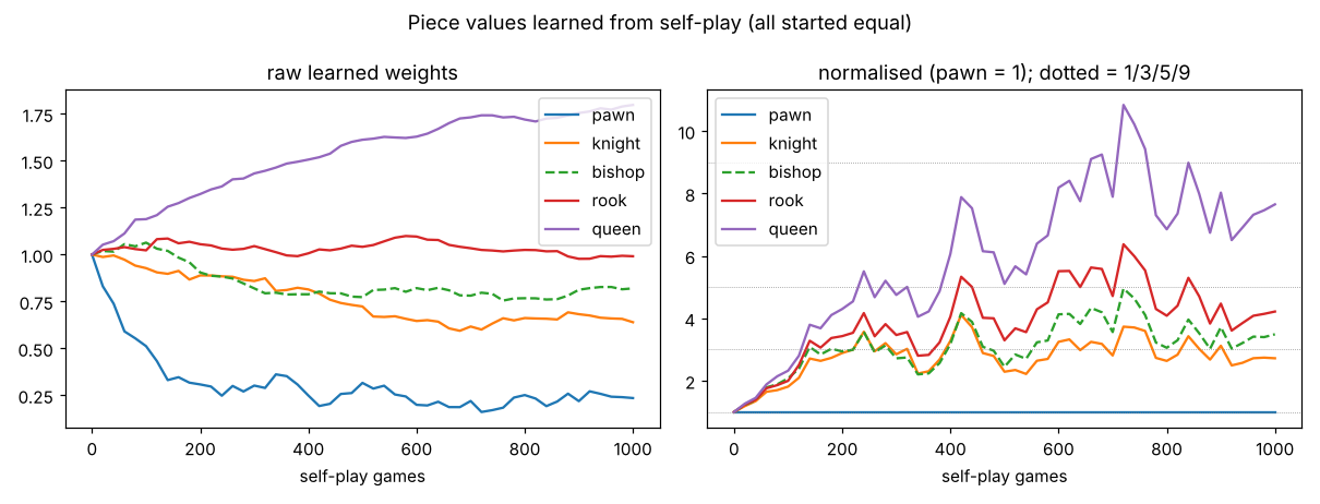
Training runs in two stages. Stage 1 learns only the piece values, from an equal start, over 1000 games. Stage 2 freezes those values and learns the 12 positional weights from zero over 300 more games. A boolean mask decides which weights the update may touch.
    if args.stage == "material":
        init = equal_material_weights(1.0)
        mask = [i < N_MATERIAL for i in range(N_FEATURES)]
        positional = False
    else:
        init_path = args.init or os.path.join(args.out, f"material{tag}.json")
        if not os.path.exists(init_path):
            init_path = os.path.join(WEIGHTS_DIR, "material.json")
        init = load_weights(init_path)
        init = init[:N_MATERIAL] + [0.0] * (N_FEATURES - N_MATERIAL)
        mask = [args.joint or i >= N_MATERIAL for i in range(N_FEATURES)]
positional = True- Stage 1: every piece starts at 1.0 and only the first 5 weights are trainable.
- Stage 2 keeps the learned material values and resets all positional weights to 0.
- Now only the positional weights train, unless
--jointalso unfreezes material.
With a step size that only decays slowly, raw TD weights keep jittering around their fixed point. The shipped weights are therefore an average over the last quarter of the checkpoints, saved every 20 games (Polyak-style averaging).
def average_checkpoints(checkpoints: List[Dict], frac: float) -> List[float]:
    """Polyak-style average of the last `frac` of the checkpoints.  Self-play
    TD with a constant-ish step size keeps jittering around its fixed point;
    averaging the tail gives a much less noisy estimate."""
    tail = checkpoints[1:] if len(checkpoints) > 1 else checkpoints
    k = max(1, int(round(len(tail) * frac)))
    tail = tail[-k:]
return [sum(c["weights"][n] for c in tail) / len(tail) for n in ALL_FEATURES]- Keep the last 25% of checkpoints and average each weight. This gives the shipped values P 0.238, N 0.662, B 0.794, R 1.001, Q 1.751, which is 1 / 2.79 / 3.34 / 4.21 / 7.37 in pawns.
A game that hits 300 plies is scored as a plain draw. Deciding it by counting textbook material would leak 1/3/3/5/9 into the learner. Of the 1000 stage-1 games, 794 ended in checkmate, so the signal comes from real results.
Turn games into a ladder
Bradley–Terry Elo by minorise–maximise
To show that each upgrade (learned values, search, positional features) adds strength, levels L0 to L3 play a round robin from random 4-ply openings with colours swapped. The results are fitted with a Bradley–Terry model, the logistic model behind Elo ratings, using Hunter’s minorise–maximise iteration (Hunter 2004). A draw counts as half a win, and L0 is anchored at 0.
    for i in range(n):
        for j in range(n):
            if i != j and cnt[i][j] > 0:
                wins[i][j] += prior_draws * 0.5
                cnt[i][j] += prior_draws
    # Minorise-maximise iterations for Bradley-Terry strengths gamma_i
    # (Hunter 2004):  gamma_i <- W_i / sum_j n_ij / (gamma_i + gamma_j).
    gamma = [1.0] * n
    for _ in range(iters):
        new = []
        for i in range(n):
            w_i = sum(wins[i])
            denom = sum(cnt[i][j] / (gamma[i] + gamma[j]) for j in range(n) if j != i)
            new.append(w_i / denom if denom > 0 else gamma[i])
        g = math.exp(sum(math.log(x) for x in new) / n)     # fix the scale
        new = [x / g for x in new]
        if max(abs(a - b) for a, b in zip(new, gamma)) < 1e-10:
            gamma = new
            break
        gamma = new
    r = [400.0 * math.log10(x) for x in gamma]
    a = r[idx[anchor]]
return {nm: r[idx[nm]] - a for nm in names}- Each pair that met gets one virtual drawn game. Without it, a bot that won every game would get an infinite rating; with it, the gaps shrink a little.
- The MM update: a player’s strength is its points divided by a sum over opponents of games played over combined strength. Each step is guaranteed not to lower the likelihood.
- Strengths only matter up to a constant factor, so they are rescaled to geometric mean 1 every iteration.
- Convert to the Elo scale (400 · log10) and anchor the random player at 0.
L0 random 0, L1 learned material at 1 ply +207, L2 depth-3 search +424, L3 positional weights +672, from 8 games per pair. These ratings only mean something inside this ladder.
The same engine in the browser
A JavaScript port that visits the same tree
GitHub Pages can’t run Python, so the board on the project page uses web/engine.js, a from-scratch port of the move generator, the 17 features and the search. The goal was more than “plays similar chess”: on a few hundred test positions it returns the same move, score and node count as engine.py. That only works if moves come out in the same order as in python-chess, because alpha-beta’s cutoffs depend on order.
  Board.prototype.legalMoves = function () {
    var ps = this._pseudo(_pseudoBuf), out = [], i;
    var inCheck = this.isCheck();
    if (!inCheck) {
      for (i = 0; i < ps.length; i++) if (this._legalAfter(ps[i])) out.push(ps[i]);
      return out;
    }
    var k = this.kingSq[this.turn], rest = [];
    for (i = 0; i < ps.length; i++) {
      var m = ps[i];
      if (this.isCastling(m)) continue;
      if (!this._legalAfter(m)) continue;
      if (mFrom(m) === k) out.push(m); else rest.push(m);
    }
    return out.concat(rest);
};- Pseudo-legal moves are generated in python-chess’s order, and each is kept if the own king is not attacked after making it.
- In check, python-chess generates king moves first, then the rest. The port reproduces that, so the stable sort in the search gives the same ties.
  Evaluator.prototype.whiteEval = function (b) {
    // Python's sum() over floats (CPython >= 3.12) uses Neumaier compensated
    // summation; reproduce it so scores match engine.py to the last bit.
    var f = features(b, this.usePositional), w = this.w;
    var s = 0 + w[0] * f[0], c = 0.0;
    for (var i = 1; i < N_FEATURES; i++) {
      var x = w[i] * f[i], t = s + x;
      if (Math.abs(s) >= Math.abs(x)) c += (s - t) + x; else c += (x - t) + s;
      s = t;
    }
    if (c && isFinite(c)) s += c;
    return s;
};- Python’s
sum()over floats uses Neumaier compensated summation (CPython 3.12 and later). A naive JavaScript loop would differ in the last bit, and a single bit can flip a comparison in the search. - The compensation term
ccollects the rounding error of each addition and is added back at the end, as CPython does.
  /* worker from a Blob URL (works from file:// and https) */
  const workerSrc='var C=('+selfplayChessModule.toString()+')();var W='+JSON.stringify(W)+';'+
    'onmessage=function(e){var d=e.data,t=performance.now();var r=C.chooseMove(d.level,W,d.moves);'+
    'postMessage({id:d.id,r:r,ms:performance.now()-t});};';
  let worker=null;
  function makeWorker(){
    try{
      const url=URL.createObjectURL(new Blob([workerSrc],{type:'text/javascript'}));
const w=new Worker(url);- The whole engine module is turned into source text with
toString(), with the weights inlined, so the search runs in a Web Worker and the board stays responsive while the bot thinks. - A Blob URL avoids a separate worker file, so the page works from
file://as well as over https.
The levels
Three knobs, one at a time
A round robin turns three knobs into an Elo ladder:
- Data: how many self-play games the weights were trained on.
- Representation: material only, or material plus positional features.
- Test-time compute: search depth.
| Level | What it is | What changed |
|---|---|---|
| L0 | Random legal move | Nothing learned, no search |
| L1 | Learned material values, 1-ply greedy (no quiescence) | + learned evaluation (stage 1, 1000 games) |
| L2 | Same values, depth-3 alpha-beta + quiescence + transposition table | + search (test-time compute) |
| L3 | L2 + 12 learned positional weights | + representation (stage 2, 300 more games) |
| L4 | AlphaZero: deep network + MCTS, trained by self-play. Described here, not implemented | + learned features and learned search policy |
L4, AlphaZero (Silver et al., 2018). AlphaZero replaces my 17 hand-chosen features with a deep residual network. The network takes the raw board and outputs a value (expected result) and a policy (a prior over moves). It also replaces alpha-beta with Monte-Carlo Tree Search (MCTS), which the policy guides. Training is still pure self-play. MCTS visit counts become the policy target, and game outcomes become the value target. So the search improves the policy, and the policy improves the search. L1 to L3 are the 1990s version of the same three ingredients (self-play data, an evaluation function, search), with a 17-parameter linear model instead of a network with millions of parameters. That is why it trains in minutes on a CPU, and also why it stays weak: a human club player would beat L3.
L2 and L3 stop after 20,000 nodes per move, as in the ladder. In the browser port that takes well under a second.
Results
From my own runs, seed 0, shipped in weights/ and results/
Stage 1: piece values from equal starting values
1000 games in 859 s. The raw shipped weights (tail-averaged) are P 0.238, N 0.662, B 0.794, R 1.001, Q 1.751. Normalised so that pawn = 1:
| Games | Pawn | Knight | Bishop | Rook | Queen |
|---|---|---|---|---|---|
| 0 | 1 | 1.00 | 1.00 | 1.00 | 1.00 |
| 20 | 1 | 1.19 | 1.23 | 1.23 | 1.27 |
| 100 | 1 | 1.81 | 2.08 | 2.00 | 2.32 |
| 200 | 1 | 2.89 | 2.94 | 3.43 | 4.30 |
| 500 | 1 | 2.29 | 2.45 | 3.30 | 5.10 |
| 1000 (last iterate) | 1 | 2.72 | 3.49 | 4.22 | 7.65 |
| Shipped (avg of last 25%) | 1 | 2.79 | 3.34 | 4.21 | 7.37 |
| Textbook | 1 | 3 | 3 | 5 | 9 |
Self-play results: 375 White wins, 419 Black wins, 206 draws. Mean game length was 128 plies. What to notice:
- The ordering emerges fast (after about 20 games). The ratios take hundreds of games and stay noisy.
- The pawn weight is what moves the most. It drops from 1.0 to about 0.24, while the rook stays near 1. Because everything is divided by the pawn weight, the normalised curves wobble with it.
- Rook and queen come out lower than the textbook values, and the bishop is clearly ahead of the knight. That is a reasonable answer for this player population: shallow, partly random players.
- A second data point: an earlier 600-game run with a constant learning rate and no averaging ended at 2.27 / 3.24 / 4.16 / 6.20 (last iterate). Same ordering, different numbers.
- A 120-game
--quickrun is too short. It ended at P 1, N 2.59, B 3.09, R 2.85, Q 3.37, with rook below bishop.
Stage 2: positional weights
300 games in 487 s, with material frozen. These are in pawns per unit of each feature (weights/positional.json):
| Feature | Weight | Feature | Weight |
|---|---|---|---|
| Mobility (per 10 squares) | +0.83 | Bishop pair | +0.05 |
| Pawn advance (per 5 ranks) | +0.35 | Isolated pawn | +0.04 |
| Rook on open file | +0.31 | King centre | −0.01 |
| Passed pawn | +0.30 | Doubled pawn | −0.06 |
| Queen centre | +0.10 | Bishop centre | −0.07 |
| Knight centre | +0.05 | King shield | −0.11 |
- Sensible signs: mobility, advanced and passed pawns, rooks on open files, and doubled pawns.
- Wrong signs, but small: isolated pawns (+0.04) and king shield (−0.11). These are what the weak self-play population taught, and I am reporting them as learned.
- Centralisation weights are tiny. Mobility already captures most of what "centralised" means. The heatmaps show the combined effect as a piece-square table.
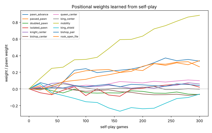
weights/positional_weights.png).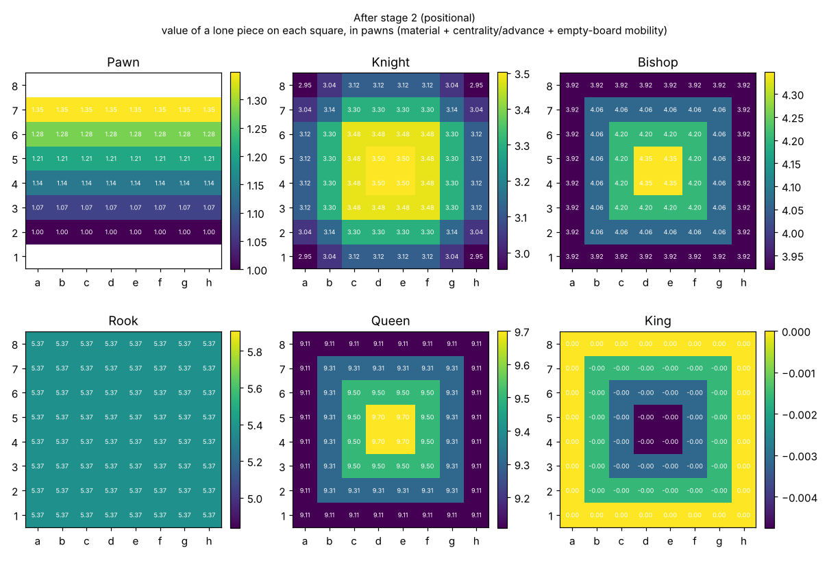
weights/positional_heatmaps.png).Ladder: round robin
8 games per pair, random 4-ply openings with colours swapped, 208 s. Rows are the player whose points are shown:
| Row vs column | L0 | L1 | L2 | L3 | Elo |
|---|---|---|---|---|---|
| L0-random | – | 1.5/8 | 0/8 | 0/8 | 0 |
| L1-material-1ply | 6.5/8 | – | 1.5/8 | 0/8 | +207 |
| L2-material-d3 | 8/8 | 6.5/8 | – | 1/8 | +424 |
| L3-positional-d3 | 8/8 | 8/8 | 7/8 | – | +672 |
How the 48 games ended: 38 checkmates, 4 adjudicated, 3 threefold repetitions, 3 reached the move cap. A game that reaches 200 plies is adjudicated as a win if one side leads by at least 3 pawns in textbook material, and otherwise as a draw. This referee rule is used in tournaments only. The --quick ladder (2 games per pair) gave the same ordering: 0 / 159 / 303 / 462.
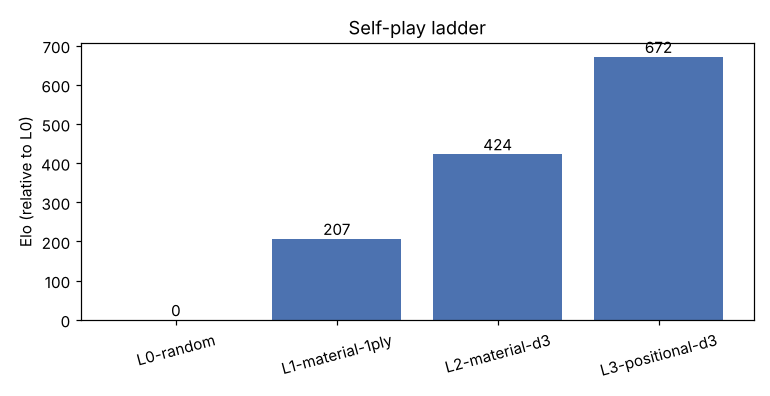
results/ladder_elo.png).Knob grid: training × search depth
Score against a fixed reference bot, 24 games per cell, 606 s. The reference is ref-textbook-d1: textbook 1/3/3/5/9 values, 1 ply + quiescence. Rows are checkpoints along the whole pipeline: material-only after g games, then positional after 1000 + g games.
| Self-play games | Depth 1 | Depth 2 | Depth 3 |
|---|---|---|---|
| 0 (material) | 0.27 | 0.29 | 0.42 |
| 20 (material) | 0.52 | 0.54 | 0.60 |
| 100 (material) | 0.52 | 0.50 | 0.58 |
| 1000 (material) | 0.52 | 0.56 | 0.58 |
| 1000+20 (positional) | 0.81 | 0.96 | 0.94 |
| 1000+100 (positional) | 0.83 | 1.00 | 1.00 |
| 1000+300 (positional) | 0.85 | 0.98 | 1.00 |
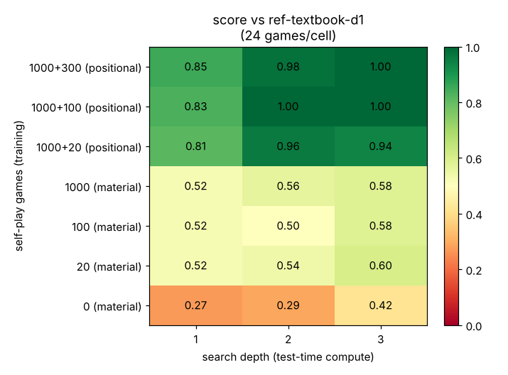
results/knob_grid.png).The default run, with 8 games per cell, gave the same picture. How to read it:
- Search partly substitutes for training. The untrained engine with all values equal gains 0.27 → 0.42 by searching to depth 3, which closes about 60% of its gap to the trained engine at depth 1 (0.52).
- The material-only rows go flat after about 20 games. A deterministic material-only searcher's choices depend mostly on the ordering of piece values, and that ordering is learned almost immediately. Many cells share identical games for this reason.
- Representation wins by far here. Adding positional features, even after only 20 stage-2 games, beats any amount of material training or depth. Depth then turns that into near-100% scores.
- Noise: with 24 games per cell, one cell's standard error is up to about ±0.10.
Train compute vs test-time compute
Andy L. Jones, Scaling Scaling Laws with Board Games (2021), trained AlphaZero agents on Hex at many sizes and found a smooth trade-off: extra train-time compute can replace test-time search, and vice versa. Roughly, each 10× of training compute could replace about 15× of test-time compute in his setting. The knob grid above is a toy, qualitative version of the same question on a much weaker system. Don't read scaling laws into a 7×3 grid.
Limits
Honest caveats
- Only one training seed is shipped, plus one earlier run with different settings. Piece-value ratios vary from run to run, and the ordering has been the stable part.
- The pawn weight shrinks a lot during training. Every number normalised by pawn value is therefore noisy. Compare the raw weights or the tail average, not single checkpoints.
- Self-play learns values for the population it plays in: 1-ply, ε-random players. The values (bishop > knight, rook ≈ 4.2) and some positional signs reflect that population, not master chess.
- Elo numbers come from 8 games per pair. They are shrunk by the virtual-draw prior, rely on material adjudication at the move cap, and only mean anything within this ladder. They are not FIDE or online ratings.
- The Python search runs at roughly 20–60k nodes per second. L2 and L3 use a 20k-node-per-move cap. L3 sometimes makes horrible moves that any club player would punish.
- What the engine leaves out: the quiescence search's stand-pat ignores stalemate; there are no null-move, killer or history heuristics; and there is no opening book.
Reproduce
CPU only: numpy, matplotlib and python-chess
Pretrained weights are included, so play.py works right away. On some Debian/Ubuntu Pythons, pip install --use-pep517 chess fixes a python-chess build error.
pip install -r requirements.txt
python play.py                         # play L2 in the terminal
python play.py --level L3 --color black
python learn.py material               # stage 1, about 14 minutes
python learn.py positional             # stage 2, about 8 minutes
                                       # (--quick for smoke tests, --out to keep the shipped weights)
python ladder.py ladder                # round robin and Elo
python ladder.py grid                  # knob grid
python -m pytest                       # 29 tests
References
Papers the method draws on
- R. S. Sutton (1988). Learning to predict by the methods of temporal differences. Machine Learning 3, 9–44.
- G. Tesauro (1995). Temporal difference learning and TD-Gammon. Communications of the ACM 38(3).
- D. F. Beal and M. C. Smith (1997). Learning piece values using temporal differences. ICCA Journal 20(3).
- J. Baxter, A. Tridgell and L. Weaver (2000). Learning to play chess using temporal differences. Machine Learning 40(3), 243–263.
- D. Silver et al. (2018). A general reinforcement learning algorithm that masters chess, shogi, and Go through self-play. Science 362(6419), 1140–1144.
- A. L. Jones (2021). Scaling Scaling Laws with Board Games. arXiv:2104.03113.
- D. R. Hunter (2004). MM algorithms for generalized Bradley–Terry models. Annals of Statistics 32(1), 384–406.
Read further
Where everything lives
- engine.py features, linear evaluator, alpha-beta search, heatmaps
- learn.py TD-Leaf(λ) self-play training, both stages, plots
- ladder.py levels L0–L3, game runner, Elo fit, ladder and knob grid
- play.py terminal play with eval and PV display
- requirements.txt numpy, matplotlib, python-chess, pytest
- web/engine.js the JavaScript port used by the in-browser board
- web/weights.js the shipped weights for the browser board
- tests/test_engine.py mates in 1 and 2, legality, symmetry
- tests/test_learn.py TD update direction, hand-computed update, masking
- tests/test_ladder_play.py Elo fit and scripted play
- weights/material.json stage-1 weights
- weights/positional.json stage-2 weights
- results/ladder_games.pgn all 48 ladder games
- results/ladder_results.json ladder scores and Elo
- results/grid_results.json knob-grid scores
- README.md full write-up and every number