How it works

Robot Sumo

Two small robots, one ring, and policies trained without a single backward pass: evolution strategies just play matches and keep whatever wins. Below are the six ideas that make it work on two laptop CPU cores, each with the few lines of code that carry it.

Reinforcement learning
Evolution strategies
Physics simulation
Vectorised numpy
JavaScript port

One generation of training

Perturb24 noise vectors give 48 copies of the net, ±ε each
Pick opponentshand-coded bots and past snapshots of itself
Playabout 1,500 matches in one vectorised simulator call
Rankaverage results become centred ranks
StepAdam moves the weights toward the winners

Traction decides who pushes whom

A small, batched physics model

Two disc-shaped, differential-drive robots share a circular ring, like the mini robot-sumo contests at maker fairs. A robot loses the moment its centre leaves the ring. If 12 seconds pass, or both leave together, it's a tie.

Sumo is a pushing game, so the one thing the simulator must get right is that a wheel can only push as hard as the floor lets it. Each 50 ms control step runs 5 substeps. Every state array has a leading dimension of n matches, so one numpy line advances all of them at once.

sumo_env.pylines 244–261

        for _ in range(SUBSTEPS):
            # motors (first-order lag)
            self.thrust_state += lag * (act[..., 0] - self.thrust_state)
            self.turn_state += lag * (act[..., 1] - self.turn_state)
            self.omega = self.turn_state * OMEGA_MAX * turn_authority

            h = np.stack([np.cos(self.heading), np.sin(self.heading)], -1)  # forward (n,2,2)
            nrm = np.stack([-h[..., 1], h[..., 0]], -1)  # left
            v_long = np.sum(self.vel * h, -1)
            v_lat = np.sum(self.vel * nrm, -1)

            # wheel/floor forces, capped by the friction circle
            f_long = F_MOTOR * self.thrust_state - DRAG * m * v_long
            f_lat = -LATERAL_GAIN * m * v_lat / dt
            f_wheel = f_long[..., None] * h + f_lat[..., None] * nrm
            f_norm = np.linalg.norm(f_wheel, axis=-1)
            scale = np.minimum(1.0, grip / np.maximum(f_norm, 1e-9))
            force = f_wheel * scale[..., None] - AIR_DRAG * m[..., None] * self.vel

Motors don't respond instantly. Each substep the actual thrust and turn move a fraction lag of the way toward the command, a first-order lag with time constant τ (50 ms by default).
Forward force is 12 N of thrust minus drag, and the sideways force tries to cancel any sliding, the way real wheels resist being pushed sideways.
The friction circle: if the combined wheel force exceeds μ·m·g, it is scaled down to that length. This one cap is why a heavier robot pushes harder and why robots skid on ice.

sumo_env.pylines 263–278

            # robot-robot spring-damper contact
            d = self.pos[:, 1] - self.pos[:, 0]  # (n,2), from robot 0 to robot 1
            dist = np.linalg.norm(d, axis=-1)
            overlap = 2 * ROBOT_RADIUS - dist
            touching = overlap > 0
            if np.any(touching):
                u = d / np.maximum(dist, 1e-9)[:, None]
                approach = -np.sum((self.vel[:, 1] - self.vel[:, 0]) * u, -1)  # >0 when closing
                fc = np.where(touching, np.maximum(0.0, K_CONTACT * overlap + C_CONTACT * approach), 0.0)
                force[:, 0] -= fc[:, None] * u
                force[:, 1] += fc[:, None] * u

            # semi-implicit Euler
            self.vel += force / m[..., None] * dt
            self.pos += self.vel * dt
            self.heading += self.omega * dt

Contact is a stiff spring with a damper (k = 3000 N/m, c = 15 N·s/m) that acts only while the discs overlap, and only pushes, never pulls.
Equal and opposite forces along the line between centres: the discs are frictionless, so contact can't twist a robot.
Semi-implicit Euler: update velocity first, then move with the new velocity. It is far more stable for a stiff spring than the naive order, and a test checks that in a head-on collision total energy only falls (within 1% wiggle) and the discs bounce apart.

See the world from your own seat

Egocentric, role-symmetric observations

Each robot sees 16 numbers, all measured in its own body frame (x forward, y left). Because the same code builds both robots' views with the roles swapped, one network can play either side, and self-play needs no special handling for “which robot am I”.

sumo_env.pylines 187–209

        out = np.empty((self.n, 2, OBS_DIM))
        for i in (0, 1):
            j = 1 - i
            c, s = np.cos(self.heading[:, i]), np.sin(self.heading[:, i])

            def rot(v):  # world -> body frame of robot i
                return np.stack([c * v[:, 0] + s * v[:, 1], -s * v[:, 0] + c * v[:, 1]], -1)

            dh = self.heading[:, j] - self.heading[:, i]
            o = out[:, i]
            o[:, 0:2] = rot(self.pos[:, j] - self.pos[:, i]) / RING_RADIUS  # opponent position
            o[:, 2:4] = rot(self.vel[:, j] - self.vel[:, i]) / VEL_SCALE  # opponent rel. velocity
            o[:, 4] = np.cos(dh)  # opponent heading, relative
            o[:, 5] = np.sin(dh)
            o[:, 6:8] = rot(self.vel[:, i]) / VEL_SCALE  # own velocity (fwd, sideways)
            o[:, 8] = self.omega[:, i] / OMEGA_MAX  # own turn rate
            o[:, 9:11] = rot(-self.pos[:, i]) / RING_RADIUS  # vector to ring center
            o[:, 11] = np.linalg.norm(self.pos[:, i], axis=-1) / RING_RADIUS  # own edge proximity
            o[:, 12] = np.linalg.norm(self.pos[:, j], axis=-1) / RING_RADIUS  # opponent's
            o[:, 13] = self.thrust_state[:, i]  # own motor states (proprioception)
            o[:, 14] = self.turn_state[:, i]
            o[:, 15] = 1.0 - self.t / MAX_STEPS  # time left
        return out

One loop for both robots: i is “me”, j is the opponent. The cosine and sine of my heading define my body frame.
Where the opponent is, rotated into my frame. A positive y means it's on my left, wherever the two robots are in the ring.
The vector to the ring centre and both robots' distances from it. This is all the network knows about the edge it must not cross.
Time left, so a policy can behave differently near the 12-second cap.

tests/test_sumo.pylines 137–148

def test_observation_swap_symmetry():
    """Swapping the two robots swaps their observations exactly."""
    rng = np.random.default_rng(1)
    n = 16
    s = random_starts(n, rng)
    s["vel"] = rng.normal(size=(n, 2, 2))
    env = SumoEnv(n)
    o0, o1 = env.reset(s)
    sw = {k: v[:, ::-1].copy() for k, v in s.items()}
    q0, q1 = SumoEnv(n).reset(sw)
    np.testing.assert_allclose(o0, q1, atol=1e-12)
    np.testing.assert_allclose(o1, q0, atol=1e-12)

Swap the two robots in the start state.
Robot 0's view of the original must equal robot 1's view of the swapped one, exactly. A sister test rotates the whole arena and checks the observations don't change.

Gradients from matches, not backprop

Evolution strategies

A match outcome (win, loss or tie) has no derivative with respect to the weights. Evolution strategies (Salimans et al. 2017) sidestep that: blur the weights with Gaussian noise, and the gradient of the average outcome can be estimated just by playing matches with noisy copies of the network, so the simulator never needs to be differentiable. The standard tricks from that paper are all here: antithetic pairs, centred-rank fitness shaping, weight decay, and Adam on the estimated gradient.

∇_θ E_ε[F(θ + σε)] = (1/σ) · E_ε[F(θ + σε) · ε]

train.pylines 66–77

def centered_ranks(x: np.ndarray) -> np.ndarray:
    """Map fitnesses to ranks scaled into [-0.5, 0.5] (ties broken arbitrarily)."""
    ranks = np.empty(len(x))
    ranks[np.argsort(x, kind="stable")] = np.arange(len(x))
    return ranks / (len(x) - 1) - 0.5


def es_gradient(fitness: np.ndarray, eps: np.ndarray, sigma: float) -> np.ndarray:
    """Antithetic ES gradient. fitness: (2P,) ordered [+eps_0..+eps_P-1, -eps_0..]."""
    r = centered_ranks(fitness)
    P = eps.shape[0]
    return (r[:P] - r[P:]) @ eps / (2 * P * sigma)

Raw fitnesses are replaced by their ranks, scaled to [−0.5, 0.5]. Only the ordering matters, so one lucky blowout win can't dominate the step, and the reward's scale stops mattering.
Antithetic pairs: each noise vector is tried as +ε and −ε, and the step uses the difference of their ranks. This cancels much of the noise in the estimate.

train.pylines 193–211

        eps = rng.standard_normal((P, N_PARAMS))
        members = np.concatenate([theta + sigma * eps, theta - sigma * eps])  # (2P, D)
        reps = 2 * P
        starts = tile_starts(random_starts(M, rng), reps)  # common random numbers
        phys = PhysParams.nominal(M)
        if dr:
            # domain randomization: most scenarios randomized, some kept nominal
            rand = PhysParams.randomized(M, rng)
            k = rng.random(M) >= cfg.get("nominal_frac", 0.0)
            for f in ("mu", "mass", "tau", "noise", "delay"):
                getattr(phys, f)[k] = getattr(rand, f)[k]
        phys = phys.tile(reps)
        env = SumoEnv(reps * M, phys, seed=int(rng.integers(1 << 31)))
        me = MLPPolicy(np.repeat(members, M, axis=0))  # env e -> member e // M
        opp = sampler.build(M, reps)
        res = run_matches(env, me, opp, rng, starts=starts)
        fit = shaped_fitness(res, shape, cfg.get("tie_penalty", 0.0)).reshape(reps, M).mean(1)
        sampler.update(res["outcome"], M)
        theta = theta + adam.step(es_gradient(fit, eps, sigma) - cfg["l2"] * theta)

The population: the current weights nudged by +σε and −σε, 48 networks in all.
Common random numbers: every member plays the same 32 start positions, so differences in fitness come from the weights, not from luck of the draw.
Each match gets its own row of weights, and the batched network evaluates all of them in one einsum per layer.
Average each member's results, turn them into a gradient estimate, subtract weight decay, and let Adam take the step.

Why not PPO

ES needs only forward passes, parallelises trivially and doesn't care that the reward arrives only at the end of a match. That fits a numpy-only, CPU-only project; the price is lower sample efficiency for large networks.

A league of past selves

Self-play with prioritized opponent sampling

Training only against your current self tends to go in circles: learn to beat strategy A, forget it, get beaten by A again. Fictitious play (Brown 1951) and fictitious self-play (Heinrich, Lanctot and Silver 2015) play against the historical mixture of past strategies instead, and L3 does a light version of this. It plays a pool: every 20 generations a snapshot joins it. Opponents are 30% hand-coded bots and 70% pool members, and the pool picks lean toward the snapshots it still struggles with (PFSP, as used in AlphaStar).

train.pylines 116–120

    def _pfsp_probs(self):
        while len(self.win_est) < len(self.pool):
            self.win_est.append(0.5)  # new snapshots start "even"
        w = (1.0 - np.array(self.win_est)) ** 2 + 0.02
        return w / w.sum()

A new snapshot starts with an estimated win rate of 0.5, so it gets a fair share of matches before the estimate settles.
Weight ∝ (1 − win rate)²: a snapshot we always beat is almost never picked, one we lose to is picked often. The small 0.02 keeps every old snapshot in rotation.

train.pylines 143–153

        pool_idx = np.full(M, -1)
        is_pool = u >= h
        n_pool = int(is_pool.sum())
        # pool share: some from the most recent snapshots, the rest by PFSP over all history
        recent = rng.random(n_pool) < self.recent_frac
        last = len(self.pool)
        k_recent = min(3, last)
        pool_idx[is_pool] = np.where(
            recent, rng.integers(last - k_recent, last, n_pool), rng.choice(last, n_pool, p=self._pfsp_probs())
        )
        kind[is_pool] = "pool"

40% of pool picks come from the three newest snapshots, to keep pressure from the current frontier.
The rest are drawn over the whole history with the PFSP weights above.

How the levels compare after training is in Results below.

Train on many worlds

Domain randomization, and a reward lesson

A policy tuned to one floor and one robot can fall apart on another. L4 continues from L3, but in 75% of its training matches the physics itself is redrawn: friction, masses, motor lag, sensor noise and observation delay. This is the main trick robotics uses to move policies from simulation to real hardware (Tobin et al. 2017; Peng et al. 2018): train on a distribution of simulators so the real world looks like one more sample.

sumo_env.pylines 81–89

    def randomized(n: int, rng: np.random.Generator) -> "PhysParams":
        """Domain randomization ranges used for training level L4."""
        return PhysParams(
            mu=np.exp(rng.uniform(np.log(0.15), np.log(1.0), n)),
            mass=rng.uniform(0.7, 2.2, (n, 2)),
            tau=np.exp(rng.uniform(np.log(0.02), np.log(0.35), (n, 2))),
            noise=rng.uniform(0.0, 0.2, (n, 2)) * (rng.random((n, 2)) < 0.6),
            delay=rng.integers(0, 3, (n, 2)),
        )

Friction from 0.15 (ice) to 1.0, drawn log-uniformly so slippery floors are not rare.
Each robot gets its own mass (0.7–2.2 kg) and motor lag (20–350 ms), so the two sides of a match can differ.
Sensor noise (σ up to 0.2) on about 60% of robots, and 0–2 control steps (0–100 ms) of observation delay.

Final evaluation is only win, loss or tie, but training adds a little shaping. L2 got up to 0.3 extra for a fast win (and lost up to 0.3 for an early loss), plus a small tiebreak for ending closer to the centre. L3 used the same shaping at 0.15, decayed to zero by generation 150. L4 uses 0.1 plus a tie penalty of 0.25.

train.pylines 91–97

    out = res["outcome"].astype(float)
    speed = 1.0 - res["end_step"] / MAX_STEPS
    d = res["final_dist"] / RING_RADIUS
    tie = out == 0
    f = out + shape * out * speed
    f[tie] = shape * np.clip(d[tie, 1] - d[tie, 0], -1, 1) - tie_penalty
    return f

A win is worth a bit more the sooner it comes; a loss hurts more the earlier it happens.
At the time cap, a small bonus for ending closer to the centre, minus tie_penalty (0.25 for L4). Final evaluation never uses any of this, only win, loss or tie.

Why the tie penalty exists

The first L4 run, scored on pure win/loss/tie, learned to hide and run out the clock: against the charger it fell from 99% wins to about 5% wins and 90% ties. Under random physics attacking is risky (on ice, a charge can carry you out of the ring), so a safe 0 looked good. The penalty was added after seeing that, so it is an honest example of reward design rather than a pre-registered experiment.

The same bots in the browser

A line-by-line JavaScript port

GitHub Pages can't run Python, so web/sim.js re-implements one match of the simulator and the policies, following the numpy code operation by operation, and web/weights.js holds the trained weights as plain arrays (1,666 numbers per level). From the same start state the port reproduces the Python trajectories to within about 10⁻⁸ m.

web/sim.jslines 288–300

    act(o) {
      let x = o;
      for (const L of this.layers) {
        const y = new Array(L.nout);
        for (let j = 0; j < L.nout; j++) {
          let s = 0;
          for (let k = 0; k < L.nin; k++) s += x[k] * L.W[k * L.nout + j];
          y[j] = Math.tanh(s + L.b[j]);
        }
        x = y;
      }
      return x;
    }

The weights are stored flat, in the same row-major order as policies.unpack, so W[k * nout + j] is entry (k, j) of the numpy matrix, and x @ W becomes this inner loop.
tanh on every layer, including the output, which keeps thrust and turn inside [−1, 1].

web/app.jslines 304–314

  /* ---------- loop: fixed 50 ms control step (25 ms at 2x) ---------- */
  let lastTs = null, raf = null, visible = true;
  function frame(ts) {
    raf = null;
    if (!st.running || !visible) { lastTs = null; draw(); return; }
    if (lastTs === null) lastTs = ts;
    const dtMs = Math.min(250, ts - lastTs); lastTs = ts;
    const stepMs = 1000 * S.CONTROL_DT / (st.mode === "bots" && st.fast ? 2 : 1);
    st.acc += dtMs;
    while (st.acc >= stepMs && st.running) { st.acc -= stepMs; step(); }
    draw(st.running ? st.acc / stepMs : 1);

The bots were trained at 20 decisions per second, so the page steps the physics in fixed 50 ms ticks (25 ms at 2× speed), whatever the screen's frame rate.
An accumulator runs as many fixed steps as real time has passed. A slow frame catches up instead of changing the physics.
Drawing gets the leftover fraction of a tick, so motion looks smooth between steps.

→

The levels

Three hand-coded bots and three trained ones

Level	What it is	How it's made
L0	Random wanderer	Holds a random (thrust, turn) for 0.5 s
L1	Charger	Hand-coded: turn to face the opponent, full throttle
Dodger	Matador	Hand-coded: sidestep when targeted, retreat from the edge, hit from the side
L2	MLP 16→32→32→2 (tanh), 1,666 weights	ES against the charger only (120 generations)
L3	Same net	ES self-play against a growing pool of its own checkpoints plus the hand-coded bots (200 generations, starting from L2)
L4	Same net	L3 continued with domain randomization of floor friction, masses, motor lag, sensor noise and delay (150 generations)

The three trained levels share one network: an MLP 16→32→32→2 with tanh, 1,666 weights. Everything trains on 2 laptop CPU cores in about half an hour.

→

Results

Shipped weights, 400 matches per cell

Score = win + ½·tie, so 0.5 means even. These numbers come from one training seed on my machine, and a different seed will give different numbers.

Round robin (row player against column player)

Row vs column	L0	L1	Dodger	L2	L3	L4
L0	0.54	0.04	0.03	0.10	0.01	0.00
L1	0.95	0.49	0.66	0.00	0.01	0.04
Dodger	0.94	0.34	0.50	0.01	0.04	0.07
L2	0.89	1.00	0.99	0.50	0.00	0.00
L3	0.98	0.99	0.95	1.00	0.50	0.50
L4	1.00	0.96	0.94	1.00	0.50	0.50

Mean score against the others: L0 0.04, L1 0.33, Dodger 0.28, L2 0.58, L3 0.89, L4 0.88.

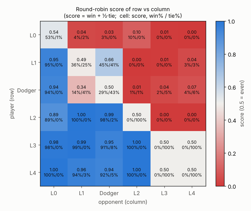
Heatmap of the round-robin scores between L0, L1, Dodger, L2, L3 and L4; the same numbers as the table above. — The round robin as a heatmap (`plots/winrate_matrix.png`).

L2 exploits the charger and is brittle against learners. It beats the charger 100% of the time and, unexpectedly, the Dodger 98% of the time, but loses every one of 400 matches against both self-play levels. It also collapses on ice (0.05 against the charger).
Self-play is broadly stronger. L3 beats every earlier level at 0.95 or above. While L3 trained, its score against L2 went from 0.5 (all ties) to 0.99 between generations 20 and 40, and it held up against the hand-coded bots.
The strongest learners draw each other. L3 vs L3, L3 vs L4 and L4 vs L4 are 100% ties: they circle near the centre and neither gives up its side. That fits the game theory, since a symmetric zero-sum game has value 0. Only a perturbation breaks the deadlock.

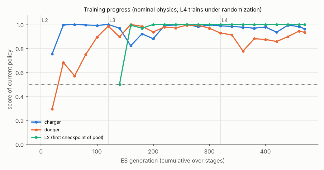
Line chart of the current policy's score against the charger, the Dodger and L2 across about 470 cumulative ES generations, with stage boundaries at L2, L3 and L4. — Training progress across the three stages (`plots/training_curves.png`).

Robustness

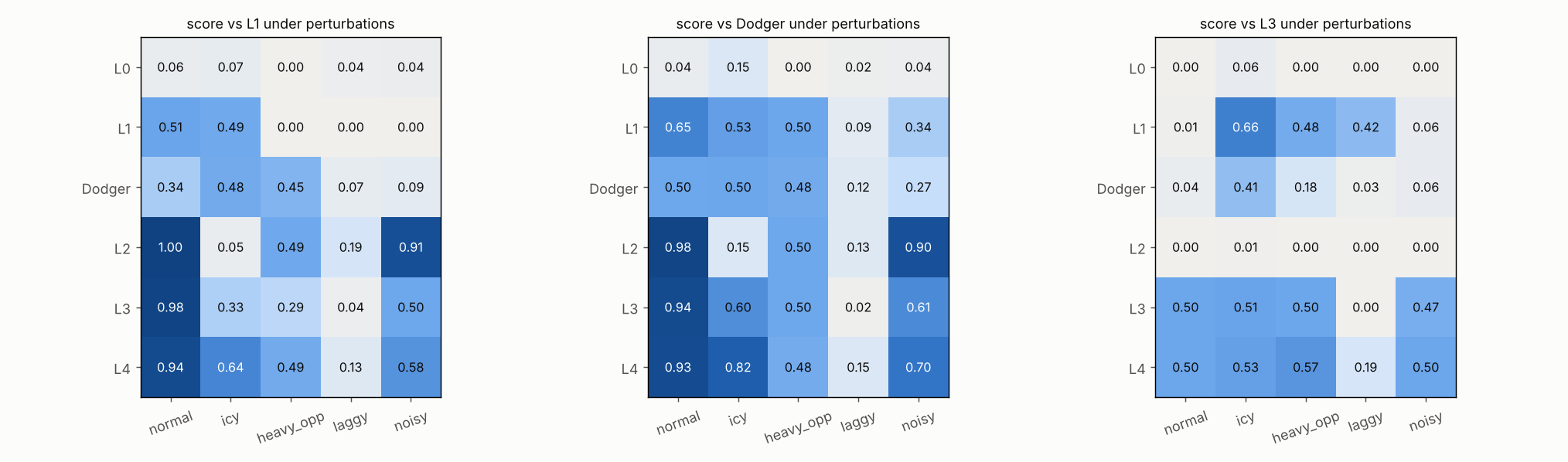
Here the level plays robot 0 against a fixed, unhandicapped opponent. Icy sets μ = 0.2 for both robots, heavy opponent gives the opponent 2 kg instead of 1 kg, laggy sets our motor lag to 300 ms with 100 ms of observation delay, and noisy adds σ = 0.15 sensor noise and 50 ms of delay to us. You can try all of these in the demo.

Against the charger	normal	icy	heavy opp.	laggy	noisy	mean
L2	1.00	0.05	0.49	0.19	0.91	0.53
L3	0.98	0.33	0.29	0.04	0.50	0.43
L4	0.94	0.64	0.49	0.13	0.58	0.56

Domain randomization helps under perturbations, partly. L4 has the best mean robustness score against all three fixed opponents (charger, Dodger and L3). The clearest gain is on ice: 0.33 → 0.64 against the charger and 0.60 → 0.82 against the Dodger. With laggy motors against L3, L4 still scores 0.19, where L3 loses to itself every time. The cost is a little nominal performance (0.98 → 0.94 against the charger).
Laggy motors remain hard for every level, and against a heavier opponent everything mostly draws, because you can't push 2 kg out with 1 kg of traction.

Three heatmaps of each level's score against the charger, the Dodger and L3 under the normal, icy, heavy opponent, laggy and noisy conditions. — Every level under every perturbation, against three opponents; tap or click to open it full size (`plots/robustness.png`).

Two matches from the Python renderer

L3 (blue) slips past the charging L1 (orange) and pushes it out of the ring. — L3 against the charger on a normal floor.

On an icy floor, L4 (blue) avoids skidding out and pushes the charger (orange) out. — L4 against the charger on ice, where L4's training on randomized physics pays off.

→

Limits

Honest caveats

The physics is a toy: frictionless discs, no wheel-level model, no ring edge lip, and a hand-tuned turning penalty on ice. It's meant to be qualitatively right (traction-limited pushing, skidding, lag), not calibrated to any real robot.
Results come from one training seed. ES and self-play are noisy, so expect different numbers, and possibly different stories, with another seed.
The Dodger heuristic is weak: it loses to the plain charger. It's there mostly as a behaviourally different opponent.
The tie penalty and shaping in L4 were added after seeing the first L4 run go passive.
Matches between learned bots are almost deterministic (the only randomness is the start position), so small gaps between nearby checkpoints can look like 0% or 100%.
In the browser, start positions, L0's commands and sensor noise come from a different random number generator than numpy's, so individual rounds differ from the Python runs even though the rules and the bots are the same.

→

Reproduce

Plain Python with numpy and matplotlib

pip install -r requirements.txt
python watch.py --human L1                            # play the charger in a window
python watch.py --p0 L4 --p1 L2 --save l4_vs_l2.gif   # render a match
python evaluate.py                                    # rebuild the tables and plots (about 2 minutes)
python train.py                                       # full retrain (about 29 minutes on 2 CPU cores)
python train.py --quick                               # 2.5-minute smoke test

→

Read further

Where everything lives

sumo_env.py vectorised simulator, physics parameters, perturbations, observations
policies.py random, charger and Dodger bots, the batched MLP, match runner
train.py ES with antithetic pairs and centred ranks, the PFSP league, L2 → L3 → L4
evaluate.py round robin, robustness tables and plots
watch.py GIF/MP4 replay, live window, human-vs-bot mode
tests/test_sumo.py physics sanity, symmetry, ES improvement, smoke tests
web/sim.js the JavaScript port used by the demo
README.md full write-up and every number
requirements.txt
results/eval.json raw win/loss/tie for every cell
weights/L2.npz, L3.npz, L4.npz shipped weights

Back to Robot Sumo All projects