How it works
Model Router
A cheap model is right most of the time; a frontier model is right more often and costs three hundred times as much. The question is which requests to send where, and how sure you can be of the answer. Below are the seven ideas behind the planner and its browser version, each with the few lines of code that carry it, then the results on the demo data, the limits and how to reproduce everything.
- Constrained optimisation
- Confidence bounds
- Calibration & holdout
- Exhaustive search
- Python → JavaScript
One run of the planner
- Splithalf the prompts tune, the other half certify
- Enumerateevery cascade on a grid of thresholds
- Pickthe cheapest one above the target, plus a margin
- Certifya lower bound on its quality from the untouched half
Cheapest cost above a quality floor
Why confidences turn routing into thresholds
The input is an eval log: a set of prompts, and for each prompt and each candidate model whether the model got it right (0 or 1, or a score between), what the call cost, and optionally how long it took and how confident the model said it was. The models run from cheap to expensive. A policy decides, request by request, which model (or models) to call. The tool looks for the policy with the lowest expected cost whose expected quality is at least a target you choose:
minimise E[cost(policy)] subject to E[quality(policy)] ≥ target
Without any signal about a request, the only policies are “always model i” and random mixtures of them, so the answer is just the cheapest single model above the floor. A confidence changes that. If a cheap model can say how sure it is, the natural policy is a cascade: call the cheapest model; if its confidence clears a threshold, keep the answer; otherwise call the next model, paying for both. For a fixed ordering, a cascade is fully described by one threshold per model, so the search space is a few numbers rather than a function of the request. Setting a threshold to “skip” drops a model from the chain, and the last model that is not skipped always answers.
    for k, i in enumerate(active):
        if not remaining.any():
            break
        rows = idx[remaining]
        cost[remaining] += log.cost[rows, i]
        if log.latency is not None:
            lat[remaining] += log.latency[rows, i]
        calls[i] = float(remaining.sum() / n)
        if k == len(active) - 1:
            acc = remaining.copy()
        else:
            acc = remaining & (conf[idx, i] >= thr[i])
        answered[acc] = i
remaining &= ~acc- Cost accumulates along the chain: every prompt still in flight pays for model i, whether or not model i ends up answering. This is what makes an unlucky cascade more expensive than the frontier model alone.
- The gate. The last active model answers everything that reaches it; the others keep a prompt only when their confidence is at least their threshold.
confis the reported confidence column, or the learned prediction from idea 03. - Prompts that were accepted leave the pool, so quality is the correctness of whichever model answered each one.
Every table in the tool starts with the single models as rows, the $0.001 model first. If the cheapest model alone meets your target, the planner says so and the cascade reduces to it.
The oracle shows the headroom
What routing could save if you knew the answers
Before searching for a policy it helps to know what any policy could possibly achieve. The oracle looks at the answers and sends each prompt to the cheapest model that got it right. Its cost is the lowest cost at which that quality can be reached, and its quality is the share of prompts that at least one model got right, which is the ceiling for every policy. The gap between the oracle and the best real policy is the price of not knowing in advance.
The oracle also traces a whole curve. Start from “cheapest model for everything”, then buy the corrections one at a time, cheapest first; each purchase moves one prompt from wrong to right at the smallest possible extra cost. For 0/1 correctness this greedy order is exactly optimal, so the curve is a hard floor under the cost–quality chart.
    best = np.full(n, -1, dtype=int)
    for i in range(m - 1, -1, -1):          # cheapest correct wins (scan expensive -> cheap)
        best = np.where(cor[:, i] >= 1.0, i, best)
    base_cost = cost[:, 0]
    base_q = cor[:, 0]
    choice = np.where(best >= 0, best, 0)
    full_cost = cost[np.arange(n), choice]
    full_q = cor[np.arange(n), choice]
    # the price of each correction, and its gain in quality
    price = full_cost - base_cost
    gain = full_q - base_q
    scale = float(log.cost.mean(axis=0).max())
    order = sorted(range(n), key=lambda j: (_key(float(price[j]), scale), -_key(float(gain[j]), 1.0), j))
    pts = [{"cost": float(base_cost.sum() / n), "quality": float(base_q.sum() / n)}]
    cs, qs = float(base_cost.sum()), float(base_q.sum())
    for j in order:
        if gain[j] <= 0:
            continue
        cs += float(price[j])
        qs += float(gain[j])
pts.append({"cost": cs / n, "quality": qs / n})- Scan the models from expensive to cheap and overwrite, so the cheapest correct model wins. Prompts no model gets right keep
-1and go to the cheapest model (they are wrong anyway). - The price of correcting each prompt and the quality it buys, sorted by price. The sort key rounds to nine digits so that numpy and JavaScript, which sum in different orders, never disagree about a tie.
- Walk the sorted list and record a point after each correction: the lower envelope of cost against quality.
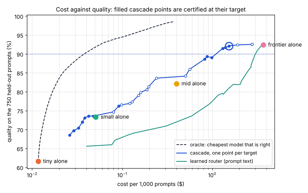
On the demo, the oracle reaches 98.5% quality for $0.374 per 1,000 prompts, against the frontier model's 92.4% for $3.69. That gap, almost ten times in cost, is the headroom. It is also a warning: 63% of prompts are answered correctly by the tiny model, but only a policy that knows which 63% can collect the saving.
Cascades against routers
Deciding after a call, or before it
A cascade decides after calling a model, using that model's own confidence. A router decides before any call, from the request alone: predict which models will be right and send the request straight to the cheapest one that looks safe. The router never pays for two calls and adds no latency, but it has less information, because “how hard is this prompt” has to be guessed from the text rather than read off the model's answer.
The tool builds both. The router's prediction is a small logistic regression per model on features of the prompt: its length, a few cues (digits, a question mark) and a hashed bag of words with 256 buckets. It is deliberately simple, so that it fits in a second and runs identically in the browser. When the eval log has no confidence column at all, the same predictions stand in as the cascade's gate, which is the classic learned router from the literature.
def evaluate_router(log: EvalLog, idx: np.ndarray, tau: float, pred: np.ndarray) -> dict:
    """Send each prompt to the cheapest model whose predicted P(correct) >= tau, else the last model."""
    n, m = len(idx), log.m
    p = pred[idx]
    ok = p >= tau
    choice = np.where(ok.any(axis=1), ok.argmax(axis=1), m - 1)
    q = log.correct[idx, choice]
    c = log.cost[idx, choice]
    return {
        "quality": float(q.sum() / n),
        "qualitySum": float(q.sum()),
        "cost": float(c.sum() / n),
"latency": float(log.latency[idx, choice].sum() / n) if log.latency is not None else None,- One threshold τ for all models: the request goes to the first (cheapest) model whose predicted chance of being right is at least τ, and to the most expensive model if none is. Because there is one number to tune, a plain grid of 64 quantiles finds the best router exactly.
- Only the chosen model is called, so quality and cost are just that model's for that prompt.
def learn_confidence(log: EvalLog, cal_idx: np.ndarray, folds: int = 5) -> np.ndarray:
    """P(model i is right | prompt text), as an (n, m) matrix.

    Calibration rows get out-of-fold predictions (fold = position in the shuffled calibration
    list mod `folds`), so the thresholds are tuned on predictions the router did not fit on.
    Every other row (the held-out split) gets the prediction of a model fit on all calibration rows.
    """
    if log.prompts is None:
        raise ValueError("learning a router needs a prompt text column")
    X = features(log.prompts)
    n, m = log.n, log.m
    pred = np.zeros((n, m))
    cal_set = np.zeros(n, dtype=bool)
    cal_set[cal_idx] = True
    for i in range(m):
        y = log.correct[:, i]
        w_all = fit_logistic(X[cal_idx], y[cal_idx])
        pred[~cal_set, i] = predict(X[~cal_set], w_all)
        for f in range(folds):
            pos = np.arange(len(cal_idx))
            test = cal_idx[pos % folds == f]
            train = cal_idx[pos % folds != f]
if len(test) == 0 or len(train) == 0:- A matrix of predictions, one column per model, covering every prompt in the file.
- Prompts in the certify half get a prediction from a model fitted on all the calibration rows, so the certify half is never used for fitting.
- Calibration rows get out-of-fold predictions: five models, each fitted on four fifths of the calibration rows and predicting the fifth it did not see. If the thresholds were tuned on in-sample predictions they would learn the regression's overconfidence, not the prompts.
Gated on reported confidence, the cascade certifies 90% quality for $1.53 per 1,000 prompts. The learned router, which only sees the prompt text, reaches the same target but has to send 97% of traffic to the frontier model to do it ($3.66). A model's own confidence is worth a lot: switching the cascade's gate to the learned predictions instead of the reported confidences, the 85% plan costs $2.33 and still misses its bound (83.5%), where the reported confidences certify 85% for $0.83.
Try every cascade
Exhaustive search with two prunings
With four models and a grid of 24 candidate thresholds per model, there are a few tens of thousands of cascades, and each can be evaluated on 750 calibration prompts in well under a millisecond. So the tool simply enumerates them all and keeps the cost and quality of every one. Two observations keep the count small: a model whose threshold accepts nothing is a wasted call, so it should be skipped instead; and a model that accepts everything left is the end of the chain, so nothing after it matters. The enumeration is a recursion over models that shares the work of the common prefix.
    def rec(i, remaining, thr, csum, qsum):
        rows_cost = float(cost_c[remaining, i].sum())
        # model i is the last active one: it answers everything that is left
        leaf(thr + [0.0] + [SKIP] * (m - i - 1), csum + rows_cost, qsum + float(cor_c[remaining, i].sum()))
        if i == m - 1:
            return
        # skip model i
        rec(i + 1, remaining, thr + [SKIP], csum, qsum)
        # or gate on a threshold
        for t in grids[i][1:]:
            acc = remaining & (conf_c[:, i] >= t)
            n_acc = int(acc.sum())
            if n_acc == 0 or n_acc == int(remaining.sum()):
                continue
            rec(i + 1, remaining & ~acc, thr + [t], csum + rows_cost, qsum + float(cor_c[acc, i].sum()))

    rec(0, np.ones(n, dtype=bool), [], 0.0, 0.0)
return thrs, np.array(costs), np.array(quals)- Option one: model i is the last one. Record a cascade right here (its threshold is written as 0, “accept all”).
- Option two: skip model i entirely and carry the same pool of prompts to the next model.
- Option three: gate on each grid threshold. A gate that passes nobody, or everybody, is dropped: both cases were covered by the first two options.
- Recurse with the prompts that escalated. The cost so far includes model i for everyone who reached it; the quality so far includes model i's answers only for the prompts it kept.
The grid is quantiles of each model's confidences on the calibration rows, plus 0. For more models the grid shrinks so that the total stays near 20,000 cascades, and a coordinate-descent pass on a finer grid polishes the result. The pick is then a sort:
def pick_best(costs, quals, target: float, scale: float):
    """Cheapest cascade with quality >= target; ties go to the higher quality, then the first
    enumerated. With no feasible cascade: the highest quality, then the cheapest."""
    ck = np.floor(np.asarray(costs, dtype=float) / scale * 1e9 + 0.5).astype(np.int64)
    qk = np.floor(np.asarray(quals, dtype=float) * 1e9 + 0.5).astype(np.int64)
    tk = _key(target, 1.0)
    feas = qk >= tk
    idx = np.arange(len(ck))
    if feas.any():
        cand = idx[feas]
        order = np.lexsort((cand, -qk[cand], ck[cand]))   # primary key last: cost, then -quality, then index
        return int(cand[order[0]]), True
    order = np.lexsort((idx, ck, -qk))
return int(order[0]), False- Costs and qualities are turned into integers (nine digits of the frontier model's cost) before comparing, so a tie is a tie in both languages.
- Among cascades whose calibration quality clears the aim, the cheapest; ties go to the higher quality, then to the first enumerated.
np.lexsorttakes its primary key last. - If nothing clears the aim, the best quality available, so the report can say how far short it falls.
Because every cascade is evaluated once, a whole sweep of targets costs nothing extra: for each target the pick is a different sort of the same list. That gives the sensitivity curve, and it also makes an exact guarantee possible: a plan that meets a higher aim also meets a lower one, so the sweep is made monotone by never paying more for less (tests/test_policies.py checks this).
Tune on one half, certify on the other
Why you cannot measure where you searched
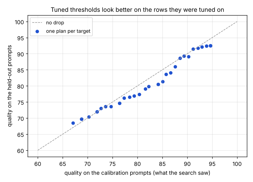
Picking the best of 9,000 cascades on 750 prompts is a form of fitting. The winner's calibration quality is optimistic: among many cascades that are truly equal, the one that happened to get lucky on these rows wins. If the same rows were then used to state a guarantee, the guarantee would inherit that luck. So the prompts are shuffled once with a seeded generator and cut in two. Thresholds are chosen on the first part only. The second part is touched exactly once, to evaluate the chosen plan, and that single evaluation is what the bound in idea 06 is computed from.
def split_indices(n: int, cal_frac: float, seed: int):
    """Shuffle 0..n-1 (Fisher-Yates) and cut: first part calibrates, the rest certifies."""
    rnd = mulberry32(seed)
    perm = list(range(n))
    for i in range(n - 1, 0, -1):
        j = int(math.floor(rnd() * (i + 1)))
        perm[i], perm[j] = perm[j], perm[i]
    k = int(math.floor(n * cal_frac + 0.5))
    k = min(max(k, 1), n - 1)
    return np.array(perm[:k], dtype=int), np.array(perm[k:], dtype=int)
- A tiny seedable generator (mulberry32) implemented in both languages, so the browser and the Python choose the same rows for the same seed.
- A Fisher–Yates shuffle; the cut point is the calibration share you choose (50% by default).
The split has a second consequence. If the plan is tuned to score exactly 90% on the calibration rows, it will typically score a little under 90% on the certify rows, and its lower bound will sit a further two points below that. So the search aims higher than the target on purpose: at the smallest observed rate that would certify the target on the certify rows, plus a safety margin of one standard error against the winner's curse.
def aim_for(target: float, n_hold: int, n_cal: int, delta: float, binary: bool, safety: float):
    """The calibration quality to tune for: the rate that certifies the target on n_hold rows, plus
    `safety` standard errors against the winner's curse of picking the best of thousands."""
    a = bounds.required_rate(target, n_hold, delta, binary)
    if a is None:
        return None
    a = a + safety * math.sqrt(a * (1.0 - a) / n_cal)
    return a if a <= 1.0 else None
- The rate to beat is computed from the size of the certify half only, never from its outcomes, so it does not use up the guarantee.
- One binomial standard error on the calibration half (adjustable in “More settings”). For the demo at 90% this means tuning to 92.9%.
A bound that is right 95% of the time
Clopper–Pearson for 0/1, Hoeffding for scores
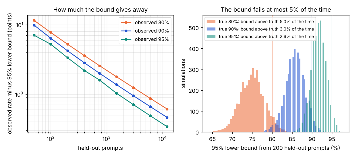
“The plan scored 92.1% on 750 held-out prompts” is a measurement with noise. The report turns it into a statement that can be acted on: with probability at least 1 − δ over the draw of those 750 prompts, the plan's true accuracy on prompts like these is at least some number. For 0/1 correctness the number is the Clopper–Pearson lower limit: the smallest true rate p under which seeing at least k successes out of n has probability δ or more. It is exact for every n (never anti-conservative), and it is a quantile of a Beta distribution, which the code computes with its own incomplete-beta function so the browser gets the same digits.
lower bound = Beta−1(δ; k, n − k + 1) certified ⇔ lower bound ≥ target
def clopper_pearson_lower(k: float, n: int, delta: float) -> float:
    """One-sided lower bound on a Bernoulli mean from k successes in n trials.

    With probability at least 1 - delta (over the random held-out sample) the true accuracy
    is above this number. k = 0 gives 0; k = n gives delta**(1/n).
    """
    if n <= 0:
        return 0.0
    k = int(math.floor(k + 0.5))
    if k <= 0:
        return 0.0
    if k >= n:
        return delta ** (1.0 / n)
return beta_ppf(delta, k, n - k + 1)- Half-up rounding, written out so Python's banker's rounding and JavaScript's
Math.roundcannot disagree. - The edge cases have closed forms: no successes gives 0; all successes gives δ1/n, which is why 750 perfect rows can certify 99.6% but not 99.8%.
- Otherwise the Beta quantile, found by 80 bisection steps on the regularised incomplete beta (Numerical Recipes' continued fraction, a Lanczos log-gamma).
tests/test_bounds.pychecks it against scipy to 10−9 and checks the coverage by simulation.
When “correct” is a score between 0 and 1 rather than a verdict, the Beta argument does not apply and the code falls back to Hoeffding's inequality: mean − √(ln(1/δ) / 2n). It is looser (about 4.5 points at n = 750, δ = 0.05, against 2 for Clopper–Pearson near 90%) but needs nothing except that scores live in [0, 1]. The same inequality, scaled by the largest possible per-prompt cost of the policy, gives the upper bound on expected cost in the table. The last piece is the message the tool gives when a target is out of reach: the rate the plan would have to show, and, if it is already above the target but not by enough, how many held-out rows would be needed at the same rate.
def required_rate(target: float, n: int, delta: float, binary: bool):
    """Smallest observed rate on n held-out rows whose lower bound still clears the target.

    This is the margin a policy must be tuned to before the held-out rows are looked at. None
    means that even a perfect score on n rows could not certify the target (too few rows).
    """
    if n <= 0:
        return None
    if not binary:
        need = target + hoeffding_radius(n, delta, 1.0)
        return need if need <= 1.0 else None
    if quality_lower_bound(n, n, delta, True) < target:
        return None
    lo, hi = 0, n          # smallest k with LB(k, n) >= target; LB is increasing in k
    while hi - lo > 1:
        mid = (lo + hi) // 2
        if quality_lower_bound(mid, n, delta, True) >= target:
            hi = mid
        else:
            lo = mid
    if quality_lower_bound(lo, n, delta, True) >= target:
hi = lo- If even n out of n would not certify the target, no plan can, and the page says so instead of searching.
- The bound rises with k, so a binary search finds the smallest number of successes that clears the target. Its rate is what idea 05 tunes towards.
The same planner in your browser
A line-for-line port, checked to nine digits
The project page runs everything in the visitor's browser: the CSV is parsed, split, searched and certified in web/router.js, a port of the Python package with the same grids, the same tie-breaking, the same random split and the same incomplete-beta function. Nothing is uploaded. The port was written to be identical, not just close: tests/parity.py runs both on five files (the demo at two targets and seeds, the learned gate, a long-layout file with fractional scores and a semicolon delimiter, and a file with no confidence column) and compares every number in the report to 10−9.
numpy evaluates a cascade with array operations over all prompts; the browser has to loop. The enumeration below is the JavaScript twin of idea 04, with a byte array for the pool of prompts still in flight:
  function enumerateCascades(log, idx, conf, grids) {
    var n = idx.length, m = log.m, thrs = [], costs = [], quals = [], i;
    var confC = [], costC = [], corC = [];
    for (i = 0; i < m; i++) { confC.push(column(log, idx, conf, i)); costC.push(column(log, idx, log.cost, i)); corC.push(column(log, idx, log.correct, i)); }

    function pad(thr, i) { var t = thr.slice(); t.push(0); for (var j = i + 1; j < m; j++) t.push(SKIP); return t; }

    function rec(i, remaining, thr, csum, qsum) {
      var rowsCost = 0, allQ = 0, nRem = 0, r;
      for (r = 0; r < n; r++) if (remaining[r]) { rowsCost += costC[i][r]; allQ += corC[i][r]; nRem++; }
      thrs.push(pad(thr, i)); costs.push((csum + rowsCost) / n); quals.push((qsum + allQ) / n);
      if (i === m - 1) return;
      rec(i + 1, remaining, thr.concat([SKIP]), csum, qsum);
      var g = grids[i];
      for (var k = 1; k < g.length; k++) {
        var t = g[k], nAcc = 0, accQ = 0, rem2 = new Uint8Array(n);
        for (r = 0; r < n; r++) {
          if (!remaining[r]) continue;
          if (confC[i][r] >= t) { nAcc++; accQ += corC[i][r]; } else rem2[r] = 1;
        }
        if (nAcc === 0 || nAcc === nRem) continue;
        rec(i + 1, rem2, thr.concat([t]), csum + rowsCost, qsum + accQ);
      }
    }
    rec(0, new Uint8Array(n).fill(1), [], 0, 0);
    return { thrs: thrs, costs: costs, quals: quals };
}- The calibration columns are copied once into flat
Float64Arrays, so the inner loops never index two levels deep. - Same leaf as the Python: model i answers everything left. Sums are plain loops, which is why idea 04 rounds before comparing.
- The same two prunings, in the same order, so the two engines enumerate the same list and “first enumerated” means the same cascade.
The one place the port had to be cleverer is the router's logistic regression. Full-batch gradient descent over 750 prompts and 261 features for 300 steps, repeated six times per model, took four seconds in a loop. The feature matrix is almost all zeros (a hashed bag of words), and skipping an exact zero changes no sum, so the port keeps each row's non-zero columns and runs in under a second with bit-identical results.
  function fitLogistic(X, y, iters, lr, l2) {
    iters = iters || 300; lr = lr || 0.5; l2 = l2 == null ? 1e-3 : l2;
    var n = X.length, d = X[0].length, w = new Float64Array(d), g = new Float64Array(d), r, j, k;
    // the hashed features are 0/1 and mostly 0: keep each row's non-zero columns (skipping exact
    // zeros changes nothing in the sums, so this stays identical to the dense numpy version)
    var nz = [];
    for (r = 0; r < n; r++) { var ix = []; for (j = 0; j < d; j++) if (X[r][j] !== 0) ix.push(j); nz.push(ix); }
    for (var it = 0; it < iters; it++) {
      g.fill(0);
      for (r = 0; r < n; r++) {
        var z = 0, x = X[r], ix2 = nz[r];
        for (k = 0; k < ix2.length; k++) { j = ix2[k]; z += x[j] * w[j]; }
        var e = 1 / (1 + Math.exp(-z)) - y[r];
        for (k = 0; k < ix2.length; k++) { j = ix2[k]; g[j] += x[j] * e; }
      }
      for (j = 0; j < d; j++) { g[j] /= n; if (j > 0) g[j] += l2 * w[j]; w[j] -= lr * g[j]; }
    }
    return w;
}- Each row's non-zero columns, found once. The first five features (bias and length cues) are dense; the other 256 are mostly empty.
- The dot product and the gradient touch only those columns. Adding
0 × wto a sum is exactly a no-op in floating point, so the result equals the dense version digit for digit. - The same update as the numpy version: divide by n, L2 on everything but the bias, step of 0.5.
The page sends the file to a Web Worker once and then re-plans every time a control moves; the learned predictions depend only on the split, so they are cached across re-plans and a slider move costs about a quarter of a second.
// Runs the planner off the main thread. The page sends the CSV text once ("load") and then
// re-plans as the sliders move ("plan"); the learned router's predictions are cached per split.
importScripts("router.js");
var log = null, predCache = {};
self.onmessage = function (e) {
  var msg = e.data, res;
  try {
    if (msg.cmd === "load") {
      log = ModelRouter.loadText(msg.text); predCache = {};
      res = { n: log.n, m: log.m, models: log.models, binary: log.binary, hasConfidence: !!log.confidence,
              hasPrompts: !!log.prompts, hasLatency: !!log.latency, warnings: log.warnings, dropped: log.dropped };
    } else if (msg.cmd === "plan") {
      if (!log) throw new Error("load a file first");
      var t0 = Date.now(), opts = msg.opts || {};
      opts.predCache = predCache;
      var rep = ModelRouter.plan(log, opts);
      rep.ms = Date.now() - t0;
      res = { report: rep, text: ModelRouter.textReport(rep, msg.unit || "$"), recipe: ModelRouter.recipe(rep), verdict: ModelRouter.verdict(rep, msg.unit || "$") };
    } else res = { error: "unknown command" };
  } catch (err) { res = { error: String(err && err.message || err) }; }
  res.id = msg.id;
  self.postMessage(res);
};
- The parsed log and the prediction cache live in the worker between messages.
- A plan request returns the full report, the text report the CLI would print, the deployment recipe and the verdict sentences.
Results
The demo data, 1,500 prompts × 4 models
The demo log is synthetic (data/make_demo.py) but shaped like a real one: prompts from nine families (arithmetic, trivia, rewriting, code, proofs, …) with a hidden difficulty shared by all models, so hard prompts are hard for everyone; prices per million tokens from $0.04 / $0.16 (tiny) to $8 / $32 (frontier), a 315× span in mean cost; confidences that are informative but noisy, with the small models over-confident. Target 90%, δ = 0.05, seed 1, 750 prompts to tune and 750 to certify.
| policy | quality | 95% lower bound | cost / 1k | latency (ms) | traffic tiny / small / mid / frontier |
|---|---|---|---|---|---|
| tiny alone | 61.6% | 58.6% | $0.012 | 228 | 100 / 0 / 0 / 0 |
| small alone | 73.3% | 70.5% | $0.051 | 465 | 0 / 100 / 0 / 0 |
| mid alone | 82.1% | 79.7% | $0.402 | 1,229 | 0 / 0 / 100 / 0 |
| frontier alone | 92.4% | 90.6% ✓ | $3.691 | 3,373 | 0 / 0 / 0 / 100 |
| Oracle | 98.5% | 97.6% | $0.374 | 629 | 63 / 23 / 9 / 5 |
| Cascade | 92.1% | 90.3% ✓ | $1.531 | 2,371 | 19 / 32 / 27 / 23 |
| Learned router | 92.7% | 90.9% ✓ | $3.660 | 3,343 | 0 / 0 / 3 / 97 |
The headline. The cascade (tiny answers if its confidence ≥ 0.970, else small if ≥ 0.916, else mid if ≥ 0.854, else frontier) is certified at 90%: on the 750 held-out prompts it scored 92.1%, with a 95% lower bound of 90.3%, at $1.53 per 1,000 prompts, 41% of the frontier model's cost and a 59% saving on the cheapest single model that is certified at this target. Every prompt starts at the tiny model; 81% go on to small, 49% to mid and 23% to the frontier. Its latency is 30% lower than the frontier's despite the extra calls, because most prompts stop early.
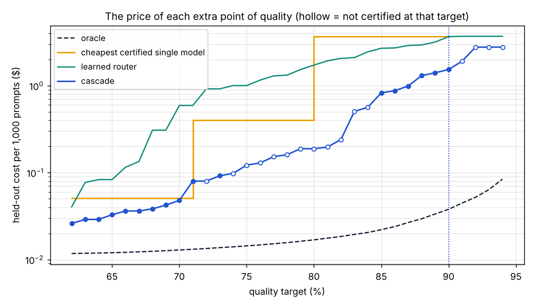
The price of each point. The sweep shows where the cascade pays off and where it stops. At targets up to 70% it certifies for $0.03–0.05, a fraction of the small model's $0.051, and tiny alone is never certified above 58.6%. Between 72% and 84% most plans scored above their target held out but their bounds fell just short (the winner's curse of idea 05; see Limits). From 85% to 90% the cascade is certified at $0.83 to $1.53, against $3.69 for the only certified single model. At 91% and above no plan clears the bound with 750 rows: certifying 91% would take about 1,200 held-out prompts at the cascade's observed rate and 92% about 7,000, and from 93% up no cascade reaches the aim even on the calibration rows (the best is 94.7%). The tool prints these numbers instead of a plan.
Safety margin and split
With the default margin of one standard error, 17 of the 33 targets in the sweep are certified on seed 1 (22 and 26 on seeds 2 and 3). Raising the margin to two standard errors certifies 28, 29 and 30 of them, at a price: the 90% plan then costs $1.91 (52% of the frontier) instead of $1.53. The 90% plan itself is certified on seeds 1 and 3 and misses on seed 2 (90.7% observed, lower bound 88.7%). Those are the honest error bars on “41%”: on this data the cascade certifies 90% for 40–60% of the frontier's cost depending on which prompts land in which half.
Browser against Python
Identical on all five parity cases, every number to 10−9: the split, the 9,081 enumerated cascades, the chosen thresholds, the bounds and the whole sweep. The browser plans the demo in about 0.75 s the first time (0.6 s of it fitting the router) and 0.25 s after that; the Python takes 2.5 s, most of it in numpy's per-cascade overhead.
Limits
What the guarantee does and does not say
- The guarantee is about prompts like these. The bound holds for the distribution the held-out prompts were drawn from. If production traffic drifts, or the eval set was curated, it says nothing. It also assumes the rows are independent: near-duplicate prompts inflate n.
- Certification is noisy near the target. A plan tuned to clear the bound by a margin can still miss it, and on the demo a band of mid-range targets did. The margin is a heuristic (one standard error of the winner's curse), not a theorem; raise it to certify more often at higher cost, or bring more rows.
- The search is exhaustive only for small sets. Four models and 24 thresholds are enumerated fully. With five or more models the grid shrinks and a coordinate pass polishes the result, which may miss the true optimum. The cascade order is fixed by mean cost.
- Confidences are taken as given. A cascade is only as good as its gate; a model that is confidently wrong defeats it, and the tool measures that rather than fixing it. Reported confidences also need to be comparable across prompts, not calibrated.
- Scores are not verdicts. With fractional scores the bound is Hoeffding (looser), and the oracle curve is greedy by price, which is exact for 0/1 scores but only approximate for fractional ones.
- The router is deliberately small. Length, a few cues and a 256-bucket hashed bag of words. A real router (an embedding model, or a fine-tuned classifier) would do better; the point here is the method, and that it runs in a second in a browser.
- Costs are what you logged. Per-prompt costs come from the file, so the cascade's cost of escalation assumes the second call costs what the eval call cost. Shared prefixes, caching and batching are not modelled, and latency is reported but never optimised.
Reproduce
Every number and figure
pip install -r requirements.txt            # numpy, scipy, matplotlib, pytest
python data/make_demo.py                   # rebuilds web/demo.csv (1,500 prompts × 4 models)
python -m router plan web/demo.csv --target 0.9 --delta 0.05     # the report above, 2.5 s
python -m router plan web/demo.csv --target 0.9 --safety 2       # the two-standard-error variant
python tools/make_figures.py               # out/*.png and the numbers quoted here, 6 s
python tests/parity.py                     # browser engine against the Python (needs node), 15 s
python -m pytest -q                        # 24 tests, about 30 s (includes the parity check)
Runtimes are wall-clock on a 2-CPU machine. Your own log: python -m router sample prints the two accepted layouts; python -m router plan your.csv --target 0.9 --json plan.json writes the full report. The project page needs only a static web server (python -m http.server from the site folder), because Web Workers do not start from file://; opened from disk it still works, on the main thread.
References
Where the ideas come from
- Clopper & Pearson (1934). The use of confidence or fiducial limits illustrated in the case of the binomial. Biometrika.
- Hoeffding (1963). Probability inequalities for sums of bounded random variables. JASA.
- Chen, Zaharia & Zou (2023). FrugalGPT: how to use large language models while reducing cost and improving performance. arXiv:2305.05176. Cascades of LLMs gated on a scorer.
- Ong, Almahairi, Wu et al. (2024). RouteLLM: learning to route LLMs with preference data. arXiv:2406.18665. Routers that decide before the call.
- Viola & Jones (2001). Rapid object detection using a boosted cascade of simple features. CVPR. The original cascade: cheap stages reject easy cases early.
- Angelopoulos, Bates, Candès, Jordan & Lei (2021). Learn then test: calibrating predictive algorithms to achieve risk control. arXiv:2110.01052. Tuning on one split and certifying with a bound on another.
- Press, Teukolsky, Vetterling & Flannery, Numerical Recipes, §6.4: the continued fraction for the incomplete beta function.
Read further
Where everything lives
- router/data.py reading both CSV layouts, column aliases, model ordering
- router/policies.py split, cascade / router / oracle evaluation, enumeration, the learned router
- router/bounds.py incomplete beta, Clopper–Pearson, Hoeffding, required rate, rows needed
- router/plan.py the whole planner: aim, sweep, certification, break-even
- router/report.py the text report, verdict sentences and deployment recipe
- router/__main__.py the command line:
python -m router plan - data/make_demo.py the synthetic eval log
- tools/make_figures.py the figures and numbers on this page
- tests/test_bounds.py against scipy, coverage by simulation
- tests/test_policies.py loading, split, evaluation against a row-by-row simulation, optimality, monotonicity, the demo headline
- tests/parity.py browser engine against the Python on five files
- requirements.txt
- web/router.js the browser engine, a port of the package
- web/worker.js runs it off the main thread
- web/page.js the project page: file loading, controls, charts, bars
- README.md the write-up and how to use it on your own log