How it works
Feedback Loop
A recommender never sees what people would have clicked on. It only sees clicks on what it chose to show, so every round of training is shaped by the previous round's choices. Below are the six ideas behind the simulator and its browser version, each with the few lines of code that carry it, then the results, the limits and how to reproduce them.
- Recommender systems
- Bandits
- Matrix factorisation
- Simulation
- Web Workers
One round of the loop
- Rankthe policy turns predicted scores into a feed of 10 per reader
- Clickreaders click by true appeal × position × boredom
- Measurediversity, coverage, Gini, value, bubble, top 1%
- Retrainthe model refits on every (shown, clicked) pair so far
Clicks are censored by what you show
Exposure bias, or data missing not at random
Imagine a feed of ten articles. You click two. The system now knows two things you liked and eight you passed over. It knows nothing at all about the 290 articles it didn't show you, and it never will unless it shows them. That is the whole problem: the training data is not a sample of what people like, it is a sample of what people like among the things the system already chose. Statisticians call this missing not at random. An item that was never shown has no clicks, which looks the same as an item nobody wanted.
The simulator makes this concrete with 300 items in eight topics, 400 readers with their own tastes, and a loop. Each round the recommender ranks, readers click, the metrics are taken, and the model is retrained on every (shown, clicked) pair so far. Readers click according to their true appeal for the item, times a position bias (the top slot gets looked at most), times 0.7n for the n-th time they have seen the same thing.
        # 1. rank: what the system believes, plus the policy's appetite for the unknown
        pred = model.scores()
        if system_discount:
            pred = pred * np.power(repeat_decay, model.N)
        pred = pred + jitter
        pred[:, ~active] = -1e9
        feeds = policies.FUNCS[pol](pred, ctx)

        # 2. clicks: true affinity x position bias x boredom with repeats, against a common coin
        shown_before = model.N[rows, feeds]
        p = world.affinity[rows, feeds] * pos[None, :] * np.power(repeat_decay, shown_before)
        base = (t - 1) * U * k
        coins = uniforms(key_click, np.arange(base, base + U * k)).reshape(U, k)
clicked = coins < p- The model's predicted click rate for every reader and item. Items nobody was ever shown come out at exactly zero (see 02).
- The recommender knows people tire of repeats, so by default it discounts an item it has already shown a reader by the same 0.7ⁿ. Switch it off in the page's settings to see a feed go stale.
- A held-back item, if any, is kept out of reach until its release round. Then the policy (01–04) turns scores into feeds.
- What readers actually do, which the system never sees directly: true appeal × 1/log₂(rank + 2) × boredom with repeats.
- One coin per (round, reader, slot), from a counter-based generator (see 06), so every policy faces the same coins.
        # 4. learn from what was shown, and only from that
        model.observe(np.repeat(np.arange(U), k), feeds.ravel(), clicked.ravel())
        ctx.item_imps += np.bincount(feeds.ravel(), minlength=M)
        ctx.total_imps += U * k
model.fit()- The only data the recommender ever gets: for each shown pair, one more impression and maybe one more click. Pairs that were not shown are not in the table at all.
- Retrain on everything so far. The next round's feeds are chosen from this model, which was fitted to the last round's feeds: that is the loop.
Round 1 has no data, so every reader gets a random feed and 100% of the catalogue is shown. In round 2 the model is little more than each item's click rate, and pure exploit shows the same 13 items to everyone: 4.3% of the catalogue, with a Gini of exposure of 0.97. From there the feed personalises and widens a little, but it never recovers: after 30 rounds pure exploit is still showing only 55% of the catalogue each round.
Collaborative filtering in a few lines
A matrix factorisation trained by alternating least squares
Collaborative filtering means guessing what you will like from what people like you liked. The classic version gives every reader a short vector pu and every item a short vector qi (six numbers each here), and predicts the click rate as a bias for the item plus the dot product pu·qi. Readers with similar vectors get similar feeds; items with similar vectors are recommended to the same people. The vectors are learned by alternating least squares: fix the items and solve for every reader (a small ridge regression each), then fix the readers and solve for every item, and repeat.
The regression is weighted by how often each pair was shown and fits the observed click rate. That weight is where the censoring enters the model.
    def fit(self) -> None:
        d, lam = self.d, self.reg
        for _ in range(self.sweeps):
            # users: solve (sum_i n_ui q_i q_i^T + lam I) p_u = sum_i (s_ui - n_ui b_i) q_i over the latent part
            Ql = self.Q[:, 1:]
            A = np.einsum("ui,id,ie->ude", self.N, Ql, Ql) + lam * np.eye(d)[None]
            b = (self.S - self.N * self.Q[:, 0][None, :]) @ Ql
            self.P[:, 1:] = np.linalg.solve(A, b[:, :, None])[:, :, 0]
            # items: solve (sum_u n_ui p_u p_u^T + lam I) q_i = sum_u s_ui p_u, bias included
            A = np.einsum("ui,ud,ue->ide", self.N, self.P, self.P) + lam * np.eye(d + 1)[None]
            b = self.S.T @ self.P
self.Q = np.linalg.solve(A, b[:, :, None])[:, :, 0]- For every reader at once: the normal-equations matrix Σ nui qiqiᵀ + λI, where nui is how often reader u was shown item i. A pair never shown has n = 0 and contributes nothing.
- The right-hand side uses the clicks sui, minus the part the item bias already explains. One batched solve gives all 400 reader vectors.
- The same for items, bias included. An item nobody has been shown has an all-zero row and column: the solve returns exactly λ⁻¹·0 = 0 for its bias and its vector, so it is predicted to be worth nothing to everyone. Pure exploit will therefore never try it. That one line is the feedback loop.
Column 0 of every reader vector is fixed at 1, so column 0 of the item vectors is the item's bias. This keeps the whole model in two arrays and two solves, and ports to JavaScript as two loops and a 7×7 Cholesky factorisation.
Explore or exploit: UCB and Thompson
The same trade-off as a multi-armed bandit, with 300 arms
Every slot in a feed is a choice between showing the item you think is best (exploit) and showing something you know little about, to find out (explore). This is exactly a multi-armed bandit, the problem in Bandits Lab: the items are the arms, an impression is a pull, a click is a reward, and the regret of pure exploitation is a catalogue you never learn about. The two classic answers transfer directly.
- Upper confidence bound. Score each item by its predicted value plus a bonus for how little it has been shown. An item seen by few people has a wide range of plausible values, so it gets a big bonus and a chance; an item that has been shown a lot and still looks poor runs out of excuses. Exploration falls out of the scoring rule.
- Thompson sampling. Instead of a bonus, add noise to each item's score in proportion to its uncertainty, and rank the noisy scores. Each item is shown roughly as often as it is plausibly the best. Randomising per reader spreads the exploration over the whole audience instead of sending everyone to the same unknown item at once.
- ε-greedy, the baseline: each slot is a random item with probability ε = 0.1. Simple, and it does find things, but it wastes most of its random slots on items the model has already seen plenty of.
def ucb(pred, ctx):
    # the bandit index: predicted score plus a bonus that shrinks with the item's exposure
    bonus = ctx.p["ucb_c"] * np.sqrt(np.log(ctx.total_imps + 1.0) / (ctx.item_imps + 1.0))
    return topk(pred + bonus[None, :], ctx.k)


def thompson(pred, ctx):
    # one posterior sample per (user, item): the score plus Gaussian noise whose spread shrinks with exposure
    U, M = pred.shape
    base = (ctx.t - 1) * U * M
    z = normals(ctx.keys["thompson"], np.arange(base, base + U * M)).reshape(U, M)
return topk(pred + ctx.p["ts_c"] * z / np.sqrt(ctx.item_imps + 1.0)[None, :], ctx.k)- UCB1's bonus with N the total impressions so far and ni the item's: c·√(log N / (ni + 1)). It is the same for every reader, so when it is large everyone is sent to the same under-shown items in the same round.
- One standard normal per (reader, item, round), drawn by counter so the Python and the JavaScript draw the same one.
- A Gaussian posterior sample: the score plus noise whose spread c/√(ni + 1) shrinks as the item is shown more. The 10 highest draws make the feed.
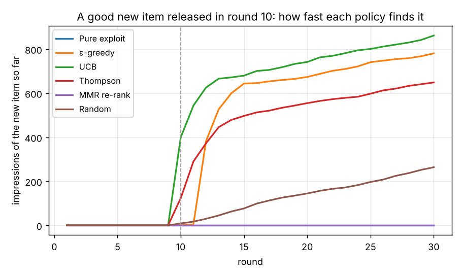
A good new item (true appeal 0.9, better than almost everything) is released in round 10. Pure exploit predicts 0 for it, like for anything with no data, and never shows it in 20 rounds. UCB shows it to all 400 readers in the round it appears and 862 times in all; Thompson sampling 649 times, spread over the rounds; ε-greedy stumbles on it twice at random, after which the model learns it is good and shows it 781 times.
Mixing the feed on purpose
Maximal marginal relevance
Exploration fixes the catalogue's problem: items that never get a chance. It does not, by itself, fix a reader's problem: a feed that is all one topic. For that there is a different tool. Maximal marginal relevance builds the feed one slot at a time, and each time picks the item with the best score minus a penalty for being too similar to what is already in the feed. Here “similar” simply means “same topic”, and the penalty is a share of the reader's top score, so it works at whatever scale the scores happen to be.
    present = np.zeros((U, T))
    work = lam * pred.copy()
    penalty = ((1.0 - lam) * pred.max(axis=1))[:, None]
    feeds = np.zeros((U, k), dtype=np.int64)
    rows = np.arange(U)
    for r in range(k):
        adj = work - penalty * present[:, ctx.topic]
        best = adj.argmax(axis=1)
        feeds[:, r] = best
        work[rows, best] = -np.inf
        present[rows, ctx.topic[best]] = 1.0
return feeds- λ = 0.7: a repeated topic costs an item 30% of this reader's best score. λ = 1 is pure exploit; λ = 0 would be eight different topics no matter what.
- For every reader at once: the adjusted score of every item, given the topics already in the feed, and the best one.
- Mark that topic as present for the next slot. Ten slots, ten passes.
MMR keeps 7–8 topics in every feed where exploit falls to 4, but it explores nothing: an item with no data still scores 0 and still never appears, so MMR's coverage (63%) is barely better than exploit's and it never shows the new item either. Diversity of the feed and diversity of the catalogue are different problems with different fixes.
Measuring a bubble
Coverage, Gini and a per-reader index
“Filter bubble” is a feeling until you count something. The simulator counts six things each round, all over the 400 simulated readers (the visitor is left out because their taste is only guessed):
- Topics per feed: distinct topics among the 10 items. Random gives about 6; the system can give at most 8.
- Coverage: the share of the catalogue that appeared in at least one feed this round.
- Gini of exposure: how unequally impressions are spread over items, 0 for perfectly even, 1 for one item taking all of them. Even a random feed scores 0.15, because 4,000 impressions over 300 items is lumpy.
- Value: the true appeal of the feed as a share of the best possible feed for that reader. The simulator knows the true appeal; the recommender does not.
- Bubble index: the share of the feed in the reader's single favourite topic, 1/8 for a random feed. Rising is partly good personalisation and partly a narrower world; the value metric is what tells the two apart.
- Top 1%: the share of all impressions that went to the three most-shown items; popularity concentration.
        f = feeds[sim]
        imps = np.bincount(f.ravel(), minlength=M).astype(float)
        imps_active = imps[active]
        topics = world.topic[f]
        distinct = np.array([len(set(row)) for row in topics])
        out["diversity"].append(float(distinct.mean()))
        out["coverage"].append(float((imps_active > 0).mean()))
        out["gini"].append(gini(imps_active))
        out["utility"].append(float((world.affinity[rows[sim], f].mean(axis=1) / best[sim]).mean()))
        out["clicks"].append(float(clicked[sim].sum(axis=1).mean()))
        out["bubble"].append(float((topics == world.top_topic[sim][:, None]).mean()))
out["top1"].append(float(np.sort(imps_active)[-n_top1:].sum() / imps_active.sum()))- Catalogue-level: how much of it was shown, and how evenly.
- Reader-level and true: mean appeal of the feed divided by the mean appeal of the 10 items that reader likes most.
- The bubble index compares each item's topic with the reader's true favourite. The top-1% share counts the heaviest 3 items.
def gini(x: np.ndarray) -> float:
    x = np.sort(np.asarray(x, dtype=float))
    n = len(x)
    s = x.sum()
    if s <= 0:
        return 0.0
    return float((2.0 * np.sum(np.arange(1, n + 1) * x)) / (n * s) - (n + 1.0) / n)
- The usual formula on sorted values: twice the rank-weighted sum over n times the total, minus (n + 1)/n.
The same run in your browser
Counter-based random numbers and a Web Worker
web/feedloop.js is a port of the four Python modules in the same order of operations: the same catalogue and names, the same readers, the same ALS, policies and metrics. The Python is numpy arrays; the JavaScript is flat Float64Arrays and loops. What makes the two agree digit for digit rather than only on average is the random number generator. Every random number is a hash of (seed, stream, counter): the click coin for round t, reader u, slot r is the same number whether numpy computes a block of 4,000 of them or the browser computes one at a time. There is no generator state to keep in step.
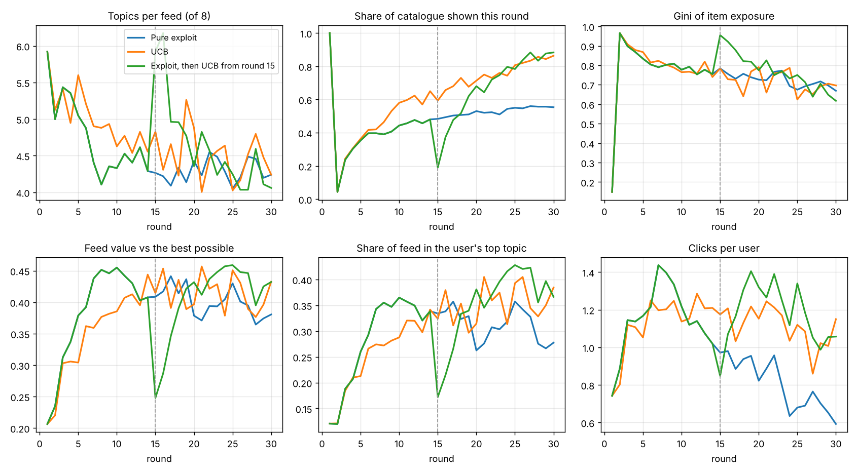
It also gives common random numbers for free. Two runs from the same seed meet the same coins, so a run that switches from exploit to UCB at round 15 is identical to the plain exploit run until round 14 and then bends; and the “new item” run differs from the plain one only where the new item is actually shown.
def hash_u32(key: int, counters) -> np.ndarray:
    c = np.asarray(counters, dtype=np.uint32)
    with np.errstate(over="ignore"):
        return _mix((c + _M3) ^ np.uint32(key))


def uniforms(key: int, counters) -> np.ndarray:
    """Uniforms in (0, 1): (h + 0.5) / 2^32, so log(u) is always finite."""
return (hash_u32(key, counters).astype(np.float64) + 0.5) / 4294967296.0- Counter plus a constant, XOR a per-stream key, then a 32-bit mixing function (two rounds of murmur-style shifts and multiplies). The JavaScript does the same with
Math.imuland>>> 0. - (h + ½)/2³² is never 0, so Box–Muller's log is always finite and the normals need no rejection loop (which would consume a data-dependent number of draws).
      var base = (t - 1) * U * k;
      for (u = 0; u < U; u++) for (r = 0; r < k; r++) {
        i = feeds[u * k + r];
        var p = world.affinity[u * M + i] * pos[r] * Math.pow(decay, model.N[u * M + i]);
        clicked[u * k + r] = uniform(keyClick, base + u * k + r) < p ? 1 : 0;
}- The click rule, one coin at a time, with the same counter arithmetic as the numpy block above. The parity test runs eight rounds of each policy on a small world in both languages and requires identical feeds, clicks and metrics.
The page runs each simulation in a Web Worker so it can draw every round as it lands. The worker steps the run one round at a time, which is also what makes the “inject exploration now” button possible: it changes the switch policy between two steps, and the resulting run is still exactly reproducible from the command line with --switch-round.
      var tick = function () {
        if (current === null || current.rn !== rn) return;
        var t = rn.step();
        postMessage({ type: "round", id: d.id, t: t, rounds: opts.rounds, metrics: rn.metrics, watched: rn.watched, newItem: newInfo,
                      switchRound: opts.switchRound || 0, switchPolicy: opts.switchPolicy || null, elapsed: Date.now() - t0 });
        if (rn.done()) {
          var res = rn.result(); res.elapsed = Date.now() - t0;
          postMessage({ type: "done", id: d.id, result: res });
          current = null;
        } else if (pace > 0) setTimeout(tick, pace);
        else tick();
};- One round: rank, click, measure, retrain. About 35 ms for 400 readers × 300 items in Chrome.
- Fast mode recurses straight into the next round; a paced run waits so a room can watch the lines grow and someone can press Inject.
Results
Seed 1, 30 rounds, 400 readers, 300 items, feeds of 10
Values in round 30, averaged over readers. Round 1 is random for every policy (5.9 topics per feed, 100% coverage, Gini 0.15).
| policy | topics / feed | coverage | Gini | value | clicks | bubble | top 1% |
|---|---|---|---|---|---|---|---|
| Pure exploit | 4.24 | 0.55 | 0.67 | 0.38 | 0.59 | 0.28 | 0.13 |
| ε-greedy (ε = 0.1) | 4.53 | 0.97 | 0.61 | 0.39 | 0.94 | 0.35 | 0.13 |
| UCB (c = 0.15) | 4.24 | 0.86 | 0.70 | 0.43 | 1.15 | 0.38 | 0.17 |
| Thompson (c = 0.3) | 4.19 | 1.00 | 0.40 | 0.41 | 0.90 | 0.37 | 0.09 |
| MMR re-rank (λ = 0.7) | 7.17 | 0.63 | 0.70 | 0.34 | 0.67 | 0.26 | 0.15 |
| Random | 6.01 | 1.00 | 0.15 | 0.20 | 0.56 | 0.13 | 0.02 |
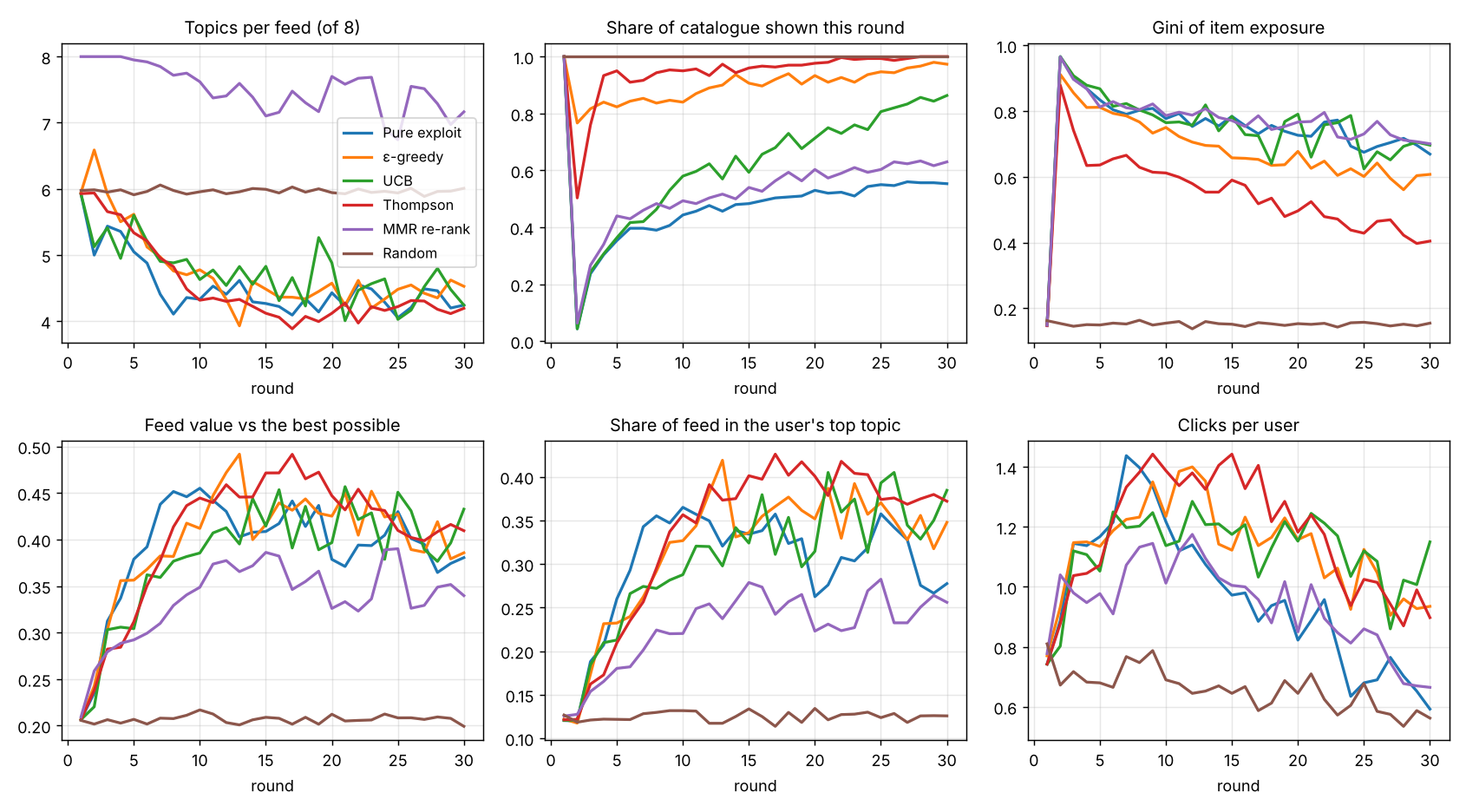
Three things stand out. First, the loop is fast: one round of data takes coverage from 100% to 4.3%, and pure exploit never gets back above 55%. Second, exploration pays for itself in the system's own currency. Pure exploit's clicks peak at 1.44 per reader around round 7 and fall to 0.59 by round 30 as it exhausts the items it knows are good and shows leftovers, while never trying the 45% of the catalogue it knows nothing about; UCB ends at 1.15 clicks and Thompson at 0.90, and both have higher true value (0.43 and 0.41 against 0.38). Third, the bandit policies do not make individual feeds more varied: they end near 4.2 topics per feed, like exploit, because they learn tastes better and lean into them (bubble 0.37–0.38 against 0.28). Only the MMR re-ranker changes that, at a cost in value. Thompson sampling spreads exposure most evenly (Gini 0.40, top 1% at 9%).
Switching policy mid-run
Pure exploit for 14 rounds, then UCB. Because the two runs share their random clicks, the curves are identical up to round 14 and then part. Coverage was 0.48 in round 14; in round 15 it drops to 0.19, because UCB's bonus for never-shown items is the same for every reader and sends everyone to the same ones at once (Gini 0.955 that round); by round 30 it is 0.88 and the Gini is 0.62, against 0.55 and 0.67 for exploit alone.
A new item, released at round 10
| policy | first shown | impressions by round 30 |
|---|---|---|
| Pure exploit | never | 0 |
| ε-greedy | round 10 | 781 |
| UCB | round 10 | 862 |
| Thompson | round 10 | 649 |
| MMR re-rank | never | 0 |
| Random | round 10 | 264 |
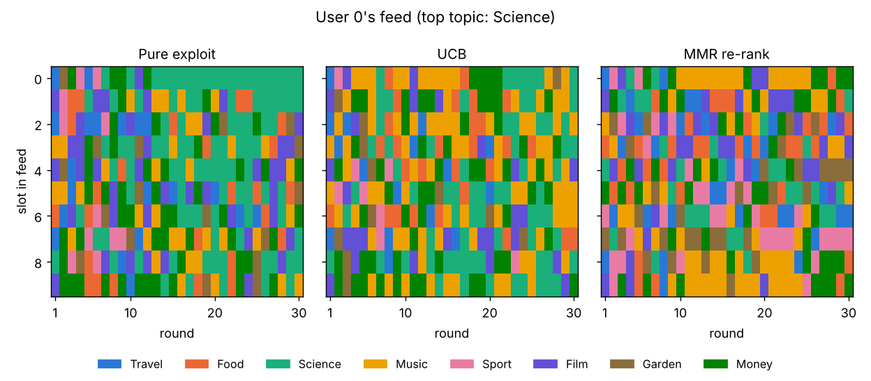
One reader's feed
Browser against the Python
The parity test runs eight rounds of exploit, ε-greedy, UCB, Thompson and MMR on a world of 80 readers and 120 items with a visitor's ratings, in both languages, and requires identical catalogue names, identical feeds and clicks for the visitor, identical impression counts for every item and metrics equal to 10⁻⁹. At full size (400 × 300, 30 rounds) exploit and Thompson also matched exactly; the browser took 1.2 s per run under node against 2.5 s for numpy.
Limits
What the numbers don't say
- It is a toy world. Tastes are fixed mixtures of eight topics, items never change, nobody joins or leaves, and the only behaviour is clicking. Real feeds have sessions, dwell time, sharing, and tastes that the feed itself shifts.
- The click model is invented. Appeal × position bias × 0.7ⁿ is plausible and standard-shaped (the position term is DCG's), but the constants are choices. Change “repeat decay” and “avoid repeats” in the page's settings and the clicks curve changes a lot; the ordering of the policies on coverage and Gini does not.
- One retrain per round, from scratch. Real systems train continuously and use side information (categories, text, images) that gives new items a non-zero score before any clicks. That softens the cold-start result but not the loop.
- The bonuses are tuned by eye. c = 0.15 for UCB and c = 0.3 for Thompson were chosen so that the bonuses are of the same order as the scores; neither is the theory's constant, which assumes rewards in [0, 1] and independent arms.
- Your taste is a guess. The visitor's twelve thumbs become their first clicks, and their later clicks are simulated from a taste guessed from those thumbs (liked topics at 1, unrated at ½, disliked near 0). The metrics leave the visitor out for that reason.
- Per-round metrics. Coverage, Gini and the top-1% share are taken per round so that a switch of policy shows up at once. Cumulative versions would be smoother and flatter.
- The seed is one world. All numbers above are for seed 1. The tests check the qualitative claims (exploit narrows, exploration widens, MMR mixes, exploit never shows the new item) on a different, smaller world.
Reproduce
Every figure and number
pip install -r requirements.txt                 # numpy, matplotlib, pytest
python -m feedloop run --policy ucb --rounds 30 --seed 1          # one policy: out/run_ucb.json + .png
python -m feedloop run --policy exploit --switch-round 15 --switch-policy ucb
python -m feedloop run --policy exploit --new-item-round 10
python -m feedloop compare --rounds 30 --seed 1                   # all of the above: ~50 s, out/compare.json + figures
python -m pytest -q                                               # 14 tests, ~5 s (needs node for the parity tests)
A single 30-round run takes about 2 s in Python. The web page prints the exact command for whatever it just ran, including --visitor with your ratings, and the two give the same numbers to every printed digit. The page needs a static web server (Web Workers don't run from file://).
References
Where the ideas come from
- Schnabel, Swaminathan, Singh, Chandak & Joachims (2016). Recommendations as treatments: debiasing learning and evaluation. ICML. (Exposure bias as missing-not-at-random data.)
- Chaney, Stewart & Engelhardt (2018). How algorithmic confounding in recommendation systems increases homogeneity and decreases utility. RecSys. (Simulating the loop.)
- Koren, Bell & Volinsky (2009). Matrix factorization techniques for recommender systems. IEEE Computer. Hu, Koren & Volinsky (2008). Collaborative filtering for implicit feedback datasets. ICDM. (ALS with confidence weights.)
- Auer, Cesa-Bianchi & Fischer (2002). Finite-time analysis of the multiarmed bandit problem. Machine Learning. (UCB1.)
- Chapelle & Li (2011). An empirical evaluation of Thompson sampling. NeurIPS. Li, Chu, Langford & Schapire (2010). A contextual-bandit approach to personalized news article recommendation. WWW.
- Carbonell & Goldstein (1998). The use of MMR, diversity-based reranking for reordering documents and producing summaries. SIGIR.
- Järvelin & Kekäläinen (2002). Cumulated gain-based evaluation of IR techniques. ACM TOIS. (The 1/log₂(rank + 2) position weight.)
- Pariser (2011). The Filter Bubble. Nguyen, Hui, Harper, Terveen & Konstan (2014). Exploring the filter bubble: the effect of using recommender systems on content diversity. WWW.
- Salmon, Moraes, Dror & Shaw (2011). Parallel random numbers: as easy as 1, 2, 3. SC. (Counter-based generators.)
Read further
Where everything lives
- feedloop/sim.py the loop: rank, click, measure, retrain; all the metrics
- feedloop/recommender.py the ALS matrix factorisation on shown pairs
- feedloop/policies.py exploit, ε-greedy, UCB, Thompson sampling, MMR, random
- feedloop/world.py catalogue, names, readers, true appeal, the visitor
- feedloop/rng.py counter-based random numbers shared with the browser
- feedloop/cli.py run and compare; the figures
- tests/test_loop.py narrowing, exploration, determinism, common random numbers, cold start, JS parity
- tests/run_js.js runs the browser engine under node for the parity test
- requirements.txt
- web/feedloop.js the port: rng, world, ALS, policies, the loop
- web/worker.js steps a run off the main thread; pacing and the live switch
- web/page.js the rating cards, the chart, the table and the feed strips
- README.md the write-up and every number