How it works
Bandits Lab
Every algorithm here answers one question: how much should you keep trying options that look worse, just in case? Below are the seven ideas that make the library and its browser version work, each with the few lines of code that carry it, then the results, the limits and how to reproduce them.
- Algorithms
- Probability & statistics
- Vectorised numpy
- Experiment design
- Web Workers
One round of play
- Selecteach policy picks an arm for every run at once
- Pullthe environment draws a reward for each pick
- Updatecounts, sums or posteriors move by one
- Scoreregret adds the gap of the arm chosen
Run a hundred worlds at once
Monte Carlo without a Python loop over runs
The problem: you repeatedly choose one of K options (“arms”) with unknown average payoffs and only see the payoff of the one you chose. Regret is how much you lose compared with always playing the best arm. Exploring costs regret now; not exploring risks getting stuck on a bad arm forever.
The Python code is a small, CPU-only library of the standard answers to that problem, written to be read, using numpy, scipy and matplotlib. Bandit results are noisy, so every number below is an average over many independent runs (100 for the main results). The slow way is a loop over runs with a loop over rounds inside it. Instead, every policy keeps its state as arrays with one row per run and one column per arm, so a single numpy operation advances all 100 runs by one round, and 100 runs of 20,000 rounds take seconds.
    def reset(self, n_runs: int, K: int, rng: np.random.Generator) -> None:
        self.R, self.K, self.rng = n_runs, K, rng
        self.counts = np.zeros((n_runs, K))
        self.sums = np.zeros((n_runs, K))
        self.t = 0  # rounds played so far
        self._rows = np.arange(n_runs)

    @property
    def means(self) -> np.ndarray:
        return self.sums / np.maximum(self.counts, 1)

    def select(self) -> np.ndarray:  # pragma: no cover - abstract
        raise NotImplementedError

    def update(self, arms: np.ndarray, rewards: np.ndarray) -> None:
        self.counts[self._rows, arms] += 1
        self.sums[self._rows, arms] += rewards
self.t += 1- The whole state of every run: how often each arm was pulled and how much it paid. Shape
(runs, arms). - Empirical means for all runs at once.
np.maximum(…, 1)avoids dividing by zero for arms not yet tried. - Fancy indexing: row r, column
arms[r]. Each run updates only the arm it actually pulled, with no loop.
    rng = np.random.default_rng(seed)
    policy.reset(n_runs, env.K, rng)
    gaps = env.gaps
    inst = np.empty((n_runs, T), dtype=np.float32)
    for t in range(T):
        arms = policy.select()
        rewards = env.pull(arms, rng)
        policy.update(arms, rewards)
inst[:, t] = gaps[arms]- The only loop is over time. Select, pull, update: the same three calls for every policy, which is why adding a new algorithm means writing just
select(and sometimesupdate). - Regret is recorded as the gap of the chosen arm, not the reward actually missed. This “pseudo-regret” has far less noise and is the quantity the theory talks about.
Be optimistic about what you don't know
UCB1 and KL-UCB
The upper-confidence-bound family scores every arm by the best value it could plausibly have, then plays the highest score. An arm that has been pulled rarely has a wide range of plausible values, so it gets a big bonus and is tried again; an arm that is truly bad eventually runs out of excuses. Exploration falls out of the scoring rule with no separate “explore” step.
    def select(self):
        rr = self._init_round_robin()
        if rr is not None:
            return rr
        bonus = np.sqrt(2.0 * np.log(self.t + 1) / self.counts)
return argmax_random_ties(self.means + bonus, self.rng)- Pull every arm once first, so no count is zero when the bonus divides by it.
- The bonus shrinks like 1/√n as an arm is pulled and grows slowly (log t) as time passes, so even a neglected arm is eventually revisited.
- Ties are broken at random rather than always picking the lowest index, which would bias early play.
UCB1's bonus is the same for every arm with the same count, so it ignores that a Bernoulli arm near 0.9 has small variance. KL-UCB replaces the square root with the tightest bound the KL divergence allows. There is no closed form for it, so the code finds it by bisection, for every run and arm simultaneously:
def klucb_index(mu, n, level, iters: int = 50):
    """Vectorized KL-UCB upper index by bisection.

    Returns max{ q in [mu, 1] : n * kl(mu, q) <= level } elementwise.
    kl(mu, .) is increasing on [mu, 1], so bisection is exact up to 2^-iters.
    """
    mu = np.asarray(mu, dtype=float)
    target = np.asarray(level, dtype=float) / np.maximum(n, 1e-12)
    lo = mu.copy()
    hi = np.ones_like(mu)
    for _ in range(iters):
        mid = 0.5 * (lo + hi)
        ok = kl_bernoulli(mu, mid) <= target
        lo = np.where(ok, mid, lo)
        hi = np.where(ok, hi, mid)
return lo # lo is always feasible- The index is the largest mean q still “consistent” with the data. Because KL only grows as q moves away from the empirical mean, a bisection search between the empirical mean and 1 finds it exactly.
- How much KL “budget” each arm has: log t spread over its n pulls. More pulls, tighter bound.
- A whole array of bisections running in lockstep:
np.wheremoves the low or high end per element. This is where KL-UCB gets its 6× lower regret than UCB1 on the five-arm instance (46.7 against 278.0 after 20,000 rounds).
Act on a sample of your beliefs
Thompson sampling
Thompson sampling keeps a full probability distribution over each arm's payoff, draws one plausible value per arm, and plays the arm whose draw is highest. An arm gets played exactly as often as it is likely to be the best. For 0/1 rewards the Beta distribution is conjugate, so “updating beliefs” is literally adding 1 to a counter.
    def select(self):
        return argmax_random_ties(self.rng.beta(self.alpha, self.beta), self.rng)

    def update(self, arms, rewards):
        binary = np.isin(rewards, (0.0, 1.0))
        r = np.where(binary, rewards, (self.rng.random(rewards.shape) < rewards))
        self.alpha[self._rows, arms] += r
        self.beta[self._rows, arms] += 1 - r
super().update(arms, rewards)- The whole decision rule: one Beta draw per (run, arm), then argmax. No tuning constant anywhere.
- Agrawal & Goyal's trick: a reward like 0.7 is turned into a coin flip that lands 1 with probability 0.7, so the posterior stays a Beta.
- Successes go to α, failures to β. Beta(α, β) narrows as evidence accumulates, which is what makes exploration fade on its own.
Thompson sampling ended at regret 28.2 against UCB1's 278.0 on the same instance after 20,000 rounds. Randomising in proportion to belief is a better use of each pull than a worst-case confidence bonus.
Measure against the floor
The Lai–Robbins lower bound
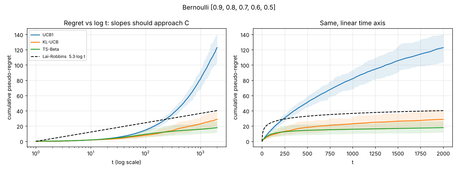
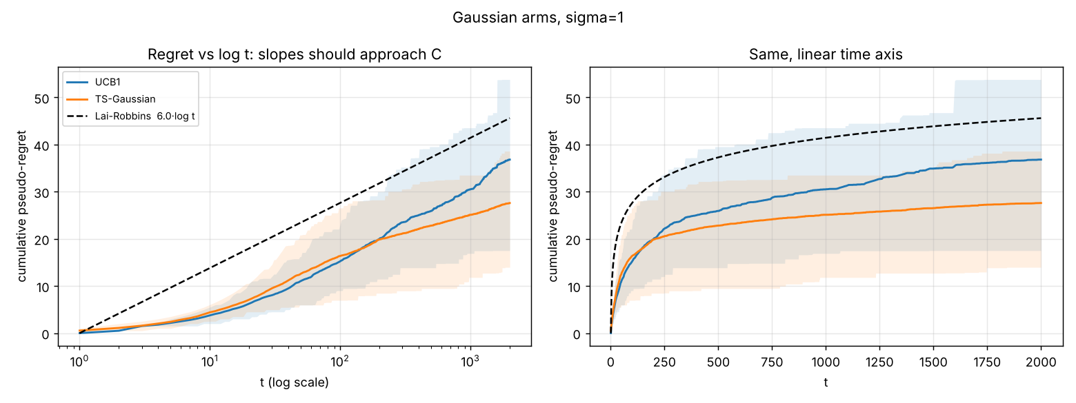
A good result needs a yardstick. Lai and Robbins proved that any reasonable policy must have regret growing at least like C · log T, and the constant C is computable from the arms' means alone. The library computes C and then fits each policy's actual slope against log t, so “near-optimal” becomes a number rather than an adjective.
C = Σi suboptimal Δi / KL(μi, μ*)
Lai and Robbins (1985) proved it for any policy that is good on every instance (“uniformly efficient”). An arm is expensive to rule out when its gap is large and it is hard to tell apart from the best arm. For the five arms 0.9, 0.8, 0.7, 0.6, 0.5, C = 5.30, so C log T = 52.5 at T = 20,000.
The bound is about the slope as T → ∞, not the height at a finite T: a good policy's curve can sit above or below C log T because of an additive constant. Over [2,000, 20,000], KL-UCB's slope against log t is 7.63 (1.44 × C) and Thompson sampling's is 3.52 (0.66 × C). Being below C at finite T doesn't contradict the bound; the local slope is still rising toward it, and finite-time curves of optimal algorithms usually look like this. UCB1 sits at 69.83 (13 × C) because its bonus ignores that Bernoulli arms near 0.9 have small variance, which KL-UCB exploits.
def lai_robbins_constant(means, kind: str = "bernoulli", sigma: float = 1.0) -> float:
    means = np.asarray(means, dtype=float)
    best = means.max()
    sub = means[means < best]
    gaps = best - sub
    if kind == "bernoulli":
        return float(np.sum(gaps / kl_bernoulli(sub, best)))
    if kind == "gaussian":
        return float(np.sum(2.0 * sigma**2 / gaps))
    raise ValueError(f"unknown kind {kind!r}")


def fitted_slope(regret_mean: np.ndarray, t_from: int) -> float:
    """Least-squares slope of mean regret against log t over t >= t_from."""
    t = np.arange(1, len(regret_mean) + 1)
    mask = t >= t_from
    x, y = np.log(t[mask]), regret_mean[mask]
return float(np.polyfit(x, y, 1)[0])- The formula above, term for term. An arm costs the most when its gap is large but its payoffs look a lot like the best arm's (small KL).
- For Gaussian arms the KL is Δ²/2σ², so each term simplifies to 2σ²/Δ.
- A straight-line fit of regret against log t, ignoring the early rounds. For the five-arm instance C = 5.3; KL-UCB's fitted slope is 1.44 × C and UCB1's is 13 × C.
Collisions as a telegraph
Multiplayer bandits with no messages
M players share K arms. If two pull the same arm they collide, both get 0, and both notice. Nobody can send messages. The team wants to spread out over the M best arms, and collective regret counts what the team loses against that. Three strategies are implemented:
- Selfish UCB. Everyone runs UCB1 on their own data and collisions are just zeros. No coordination at all.
- Musical chairs (Rosenski, Shamir & Szlak, 2016). Explore uniformly for T0 rounds, estimate M from how often you collide (
P(no collision) = (1 − 1/K)^(M−1)), then grab random arms among your estimated top M until one is free, and stay there. - SIC-style, simplified (in the spirit of SIC-MMAB, Boursier & Perchet, 2019). Orthogonalise with musical chairs on all K arms; a roll call (for each pair of seats a, b, the player on a visits b, and a collision means b is occupied) tells everyone M and a distinct rank; collision-free sequential hopping explores the candidate arms (2p pulls per arm per player in phase p); followers send their exact success counts to the leader in binary; the leader eliminates arms that have M arms confidently above them and broadcasts one bit per arm; when M arms remain, each player commits to its own.
When several players share the arms and nobody may talk, the only thing a player can observe about the others is a collision. The SIC-style protocol turns that into a communication channel: on a scheduled round, a follower either steps onto the leader's arm (a collision means bit 1) or stays put (bit 0). Since every phase length is known in advance, everyone stays in sync without a clock or a message.
                for follower in range(1, M):
                    for a in range(c):
                        value = 0
                        for b in range(n_bits):
                            bit = (int(succ[follower, a]) >> b) & 1
                            arms = np.arange(M)          # rank j waits on arm j
                            if bit:
                                arms[follower] = 0       # collide on leader's arm
                            r, occ = round_regret(arms)
                            reg.append(r)
                            value |= int(occ[0] > 1) << b  # leader decodes collision
                        received[a] += value
                emit(reg)
                assert np.array_equal(received, succ[1:].sum(axis=0))
S[Carr] += succ[0] + received- The follower reads off one binary digit of its success count for arm
a. - Bit 1: move onto arm 0, where the leader sits, on purpose. Bit 0: stay on your own arm.
- The leader sees only whether arm 0 had more than one player, and rebuilds the number bit by bit.
- Every signalling round still costs regret, and it's charged honestly. That's why the protocol's regret grows like log T rather than staying flat.
- A built-in check that what the leader decoded equals what the followers actually observed.
From theory to an A/B plan
Simulate the next four weeks before running them
The planner applies the same ideas to a real decision. Given a baseline conversion rate, plausible lifts, daily traffic and a horizon, it simulates hundreds of possible futures of your website traffic and runs three strategies on each. Traffic is reallocated once a day, because that's how often most teams can actually ship a change. All arms are Bernoulli with Beta(1, 1) priors.
- Fixed split. Equal traffic until a pre-registered sample size (two-sided two-proportion z-test, Bonferroni over variants, chosen power and minimum detectable effect), then ship a variant only if it beats control significantly, otherwise keep control. Clean, unbiased inference and the highest exploration cost.
- Thompson sampling. Daily traffic split in proportion to P(arm is best). Fewest lost conversions.
- Top-two Thompson sampling (Russo, 2016; β = ½). Built to identify the best arm; stops and ships once P(best) ≥ 0.95.
It reports expected lost conversions, how often the final choice is the true best arm, and how long it takes to reach a confident decision. If you don't give the lifts, each simulation draws them uniformly from ±max-lift, so the report averages over plausible worlds.
        else:
            post = prob_best(1 + S, 1 + N - S, rng, args.draws)
            if name == "ts":
                probs = post
                newly = np.isinf(decided) & (post.max(axis=1) >= args.confidence)
                decided[newly] = d
            else:  # ttts: stop & ship once confident
                newly = (shipped < 0) & (post.max(axis=1) >= args.confidence)
                shipped[newly] = post[newly].argmax(axis=1)
                decided[newly] = d
                probs = np.where((shipped >= 0)[:, None],
                                 np.eye(K)[np.maximum(shipped, 0)],
                                 top_two_allocation(post, args.ttts_beta))
        n = allocate(args.traffic, probs, rng)
        conv = rng.binomial(n, rates)
        S += conv
        N += n
lost[:, d] = (n * (best[:, None] - rates)).sum(axis=1) # expected loss- P(each variant is best) from Beta(1 + successes, 1 + failures) posteriors, estimated by sampling.
- Batched Thompson sampling: tomorrow's traffic split is today's probability of being best.
- Top-two TS ships the winner as soon as P(best) ≥ 95%; until then it deliberately spreads traffic between the top two contenders to separate them faster.
- The cost being compared: conversions lost by sending visitors to anything but the true best variant.
Only the fixed split gives an unbiased effect size. The bandits lose fewer conversions, but their data is collected adaptively, so a plain t-test on it is biased. The planner reports how often each strategy picks the right winner instead.
A 5% baseline with variants at +5% and +10% and 2,000 visitors a day: the fixed test would need 147,889 visitors per arm (222 days) to detect a 5% lift, so in 28 days it is badly underpowered. That one sentence is often the most useful output.
The same algorithms in your browser
A line-by-line port, run in a Web Worker
The project page runs the simulator and the planner in the visitor's browser with no server and no libraries. web/bandits.js and web/planner.js are ports of bandits/algorithms.py, bandits/lower_bound.py and tools/ab_test_planner.py: the same policies, constants, priors, ε schedule, KL-UCB definition and planner decision rules. Three things differ, and none of them changes what is computed:
- Loops instead of arrays. numpy advances all runs at once; JavaScript has no array maths, so the state lives in flat
Float64Arrays (row r, arm k atr·K + k) and a plain loop goes over the runs inside the loop over rounds. - A different random stream.
web/rng.jsis a seedable xoshiro128** generator with the same distributions as numpy (polar-method normals, Marsaglia–Tsang gammas, Beta as a ratio of gammas, inversion and Hörmann's BTRS for binomials, numpy's conditional-binomial multinomial). Results therefore agree with the Python on average, not run for run. - Faster but exact KL-UCB. The bisection is the same, written with two logs per step instead of four, and it stops early on arms that provably cannot win.
  Simulation.prototype.step = function (rounds) {
    var pol = this.policy, R = this.R, rng = this.rng, means = this.means, gaps = this.gaps;
    var gauss = this.kind === "gaussian", sigma = this.sigma;
    var end = Math.min(this.T, this.t + rounds);
    for (; this.t < end; this.t++) {
      var tot = 0;
      for (var r = 0; r < R; r++) {
        var arm = pol.select(r);
        var x = gauss ? means[arm] + sigma * rng.normal() : (rng.random() < means[arm] ? 1 : 0);
        pol.update(r, arm, x);
        tot += (this.regret[r] += gaps[arm]);
      }
      pol.endRound();
      this.meanCurve[this.t] = tot / R;
    }
return this.t >= this.T;- One round for one run: pick an arm, draw a Bernoulli (or Gaussian) reward, update. Runs are independent, so doing them one after another gives the same result as numpy doing them side by side.
- Pseudo-regret again: add the gap of the arm chosen, exactly like
inst[:, t] = gaps[arms]. - The mean over runs at every t is kept, so the page can draw the curve while the run is still going.
  function klucbIndex(mu, n, level, iters, stopBelow) { // max{q in [mu,1] : n kl(mu,q) <= level}
    // Same bisection as klucb_index (lo = mu, hi = 1). kl(mu, q) is written as
    // h(mu) - mu log q - (1-mu) log(1-q) so each step costs two logs, not four.
    var e = 1e-15, p = Math.min(Math.max(mu, e), 1 - e);
    var target = level / Math.max(n, 1e-12) - p * Math.log(p) - (1 - p) * Math.log(1 - p);
    var lo = mu, hi = 1;
    for (var i = 0; i < iters; i++) {
      var mid = 0.5 * (lo + hi), q = Math.min(Math.max(mid, e), 1 - e);
      if (-p * Math.log(q) - (1 - p) * Math.log(1 - q) <= target) lo = mid;
      else { hi = mid; if (hi <= stopBelow) return -Infinity; }
    }
    return lo;
  }
- kl(μ, q) = h(μ) − μ log q − (1 − μ) log(1 − q). The h(μ) part does not depend on q, so it is folded into the target once.
- Same 30 bisection steps from [μ, 1], same 10−15 clipping, as in the Python.
- If the bracket's top falls to the current best index, this arm's finished index would be strictly lower, so it can neither win nor tie. Stopping is safe.
      // full index for the arm this run played last, then prune the others against it
      var first = this.last[r], top = klucbIndex(this.mean[off + first], this.counts[off + first], level, 30);
      this.score[first] = top;
      for (var k = 0; k < K; k++) {
        if (k === first) continue;
        var v = klucbIndex(this.mean[off + k], this.counts[off + k], level, 30, top);
        this.score[k] = v; if (v > top) top = v;
      }
return (this.last[r] = argmaxTies(this.score, 0, K, this.rng));- Compute the full index first for the arm this run played last round; it is usually the winner, so most other arms are ruled out after a few steps. This made KL-UCB about 30% faster.
- The others are bisected only as far as needed against the best index so far.
The planner's only non-random step is the fixed test's sample size. scipy's norm.ppf is replaced by Wichura's AS241 algorithm, which is accurate to about 10−16, so the sample size and test length come out identical to the Python tool.
  function fixedSampleSize(p0, mdeRel, nVariants, alpha, power) {
    var p1 = p0 * (1 + mdeRel), a = alpha / Math.max(nVariants, 1);
    var za = normPpf(1 - a / 2), zb = normPpf(power);
    var v = p0 * (1 - p0) + p1 * (1 - p1);
    return Math.ceil((za + zb) * (za + zb) * v / ((p1 - p0) * (p1 - p0)));
}- zα/2 at the Bonferroni level and zpower. Over 16 probabilities from 10−10 to 1 − 10−9, the largest difference from scipy was 1.8 × 10⁻¹⁵.
Both tools run in a Web Worker so the page stays responsive. The worker posts progress as it goes; pressing Stop simply terminates it, so the loops never need to check a flag.
  var chunk = 20, t0 = Date.now(), t = 0;
  while (t < T) {
    var start = Date.now();
    sims.forEach(function (s) { s.step(chunk); });
    t = Math.min(T, t + chunk);
    var took = Date.now() - start;          // aim for ~40 ms between updates
    chunk = Math.max(1, Math.min(T, Math.round(chunk * Math.min(4, Math.max(0.25, 40 / Math.max(took, 1))))));
    postMessage({ type: "progress", t: t, elapsed: Date.now() - t0, curves: sims.map(function (s) { return sample(s.meanCurve, g, t); }) });
}- All chosen strategies advance by the same number of rounds, so their curves grow side by side.
- The chunk size adapts so that an update arrives about every 40 ms, whatever the horizon and however slow KL-UCB is.
- Only about 700 sample points per curve are sent (evenly spaced and log-spaced), enough for both the linear and the log-time chart.
Results
What the Python runs found
| policy | idea | regret |
|---|---|---|
| ε-greedy | explore at random with probability ε | linear for fixed ε; log T with a decaying schedule tuned to the gap |
| Explore-then-commit | m pulls per arm, then commit | needs m tuned to the gap and horizon |
| UCB1 | optimism: mean + √(2 log t / n) (Auer, Cesa-Bianchi & Fischer, 2002) | O(Σ log T / Δ), not the optimal constant |
| KL-UCB | largest q with n·KL(μ̂, q) ≤ log t (Garivier & Cappé, 2011) | matches the Lai–Robbins constant for Bernoulli arms |
| Thompson sampling | play the arm that is best under a posterior sample (Beta or Gaussian) | asymptotically optimal for Bernoulli arms |
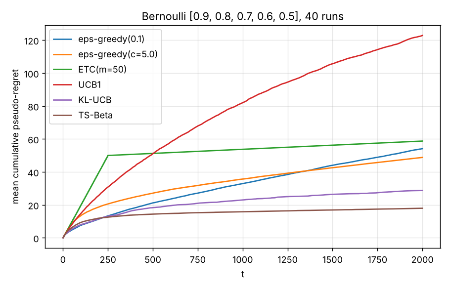
Five Bernoulli arms with means 0.9, 0.8, 0.7, 0.6, 0.5; T = 20,000; 100 runs; ± is the standard error. The Lai–Robbins bound gives C log T = 52.5.
| policy | regret at T |
|---|---|
| ε-greedy, fixed ε = 0.1 | 418.9 ± 3.9 |
| ε-greedy, decaying (c = 5) | 103.9 ± 33.7 |
| Explore-then-commit (m = 50) | 366.0 ± 72.4 |
| UCB1 | 278.0 ± 2.5 |
| KL-UCB | 46.7 ± 1.2 |
| Thompson sampling (Beta) | 28.2 ± 1.1 |
Multiplayer
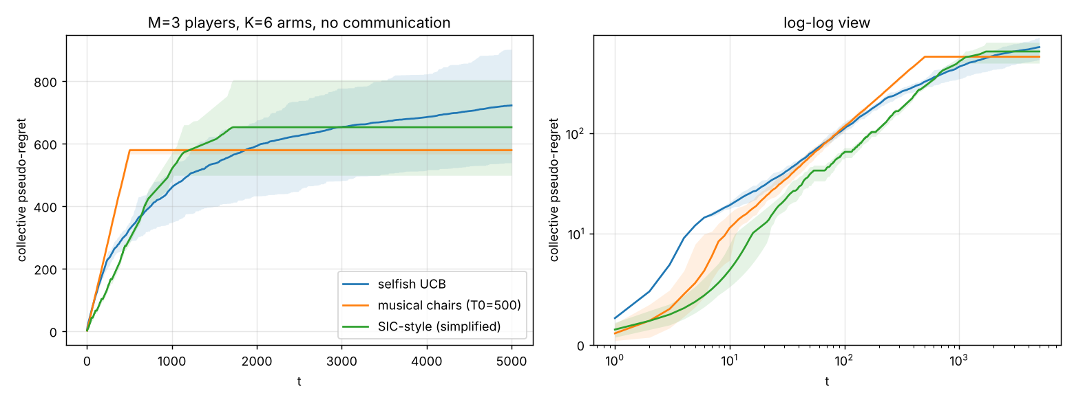
| K = 6, M = 3, T = 50,000, 30 runs | collective regret | median | collisions per run |
|---|---|---|---|
| Selfish UCB | 977.2 | 948.3 | 742 |
| Musical chairs (T0 = 1,000) | 1159.5 | 1163.1 | 929 |
| SIC-style (simplified) | 812.1 | 810.7 | — |
Arm means 0.9, 0.8, 0.7, 0.5, 0.4, 0.3. All three methods ended on the best three arms in the final round of every run, and the SIC-style protocol had no failures. SIC-style regret is flat after about 3,000 rounds and grows only with log T (683 → 793 → 888 for T = 5k, 50k, 200k; 20 runs). Musical chairs pays roughly linearly in T0. Selfish UCB keeps colliding and its regret is still growing.
A/B planner
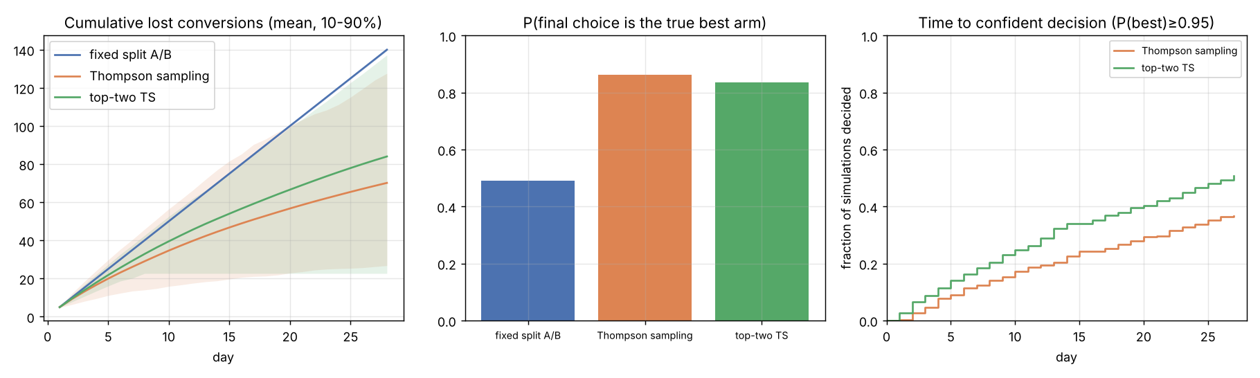
A 5% baseline with variants at +5% and +10%, 2,000 visitors a day for 28 days, 300 simulations:
| strategy | lost conversions (mean ± sd) | picks the best | decided by the end | median day decided |
|---|---|---|---|---|
| Fixed split A/B | 140.0 ± 0.5 | 49.0% | forced at end | > 28 |
| Thompson sampling | 70.1 ± 40.0 | 86.3% | 37% | 11 |
| Top-two TS | 84.0 ± 40.9 | 83.7% | 51% | 11 |
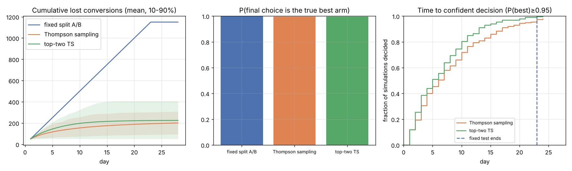
With 20,000 visitors a day (200 simulations) the fixed test fits in 23 days and picks the best arm every time, and the bandits lose only about a sixth to a fifth as many conversions: 200.4 for Thompson sampling (99.5% correct, median decision on day 6) and 224.8 for top-two TS (99.5%, day 5), against 1,150.1.
Browser port against the Python
Same instance (0.9, 0.8, 0.7, 0.6, 0.5), independent random streams, mean final regret ± standard error. Lai–Robbins constants are identical to every printed digit (C = 5.3006, C log T = 52.49 at T = 20,000; 6.0 for the Gaussian instance).
| policy | Python, T = 20,000, 300 runs | browser, same | Python, T = 2,000 | browser, same |
|---|---|---|---|---|
| ε-greedy (0.1) | 418.8 ± 2.4 | 419.4 ± 2.6 | 56.44 ± 0.32 | 56.01 ± 0.31 |
| ε-greedy, decaying | 71.1 ± 11.5 | 59.7 ± 9.5 | 36.56 ± 0.24 | 36.63 ± 0.24 |
| Explore-then-commit | 194.8 ± 31.1 | 227.7 ± 36.4 | 64.67 ± 0.35 | 65.01 ± 0.36 |
| UCB1 | 280.0 ± 1.6 | 281.5 ± 1.6 | 119.26 ± 0.05 | 119.33 ± 0.05 |
| KL-UCB | 45.2 ± 0.7 | 43.4 ± 0.7 | 27.45 ± 0.09 | 27.25 ± 0.09 |
| Thompson (Beta) | 29.2 ± 0.7 | 31.0 ± 1.6 | 20.41 ± 0.11 | 20.28 ± 0.11 |
At T = 2,000 the runs are 10,000 per policy (20,000 for ETC and decaying ε, 80,000 for UCB1). Every difference is within about 2 standard errors. As a stricter check, the deterministic policies (UCB1, KL-UCB, ETC) were fed the same table of random numbers in both languages, with ties broken by lowest index: all 100,000 arm choices matched. The planner's sample sizes matched exactly on seven inputs (e.g. 147,889 per arm for +5%, 8,155 for 5% → 6%), and its simulated columns agreed within noise (e.g. 2,000/day, +5%/+10%: Thompson sampling lost 69.6 in Python and 73.7 in the browser with per-simulation sd ≈ 40 over 300 simulations).
Limits
What the numbers don't say
- Lai–Robbins is asymptotic. At finite T a good policy can sit above or below C log T; only the slope is constrained, and it approaches C slowly.
- The A/B trade-off. Bandits minimise regret, top-two TS finds the winner fastest, and only the fixed split gives valid inference: controlled error rates, unbiased effect sizes and simple confidence intervals.
- “Confident” is Bayesian. For TS and top-two TS it means posterior P(best) ≥ 0.95 under a flat prior. Under data-dependent stopping that is not a frequentist 5% error rate; trust the simulated “picks the best” column instead.
- Adaptive data is biased. After adaptive allocation, naive conversion rates and t-tests are biased. Use the bandit to allocate traffic, and keep a fixed holdout if you need a clean effect size.
- A simple world. The planner assumes stationary conversion rates, independent visitors and immediate conversions. Real traffic has weekday effects, novelty effects and delayed conversions.
- Selfish UCB is not safe in general. It worked on this instance, but Boursier & Perchet (2019) discuss instances where it fails. Musical chairs needs T0 set from the gap.
- The SIC-style protocol is simplified. Statistics are gathered at a single leader instead of all-to-all quantised broadcasts; arms are not “accepted” early, so everyone explores until exactly M candidates remain; ranks come from O(K²) pairwise probes instead of SIC's O(K) sequential hopping; and exact integer counts are sent instead of quantised means. If orthogonalisation fails (probability ≤ 1/T by construction), the run is charged maximal regret for the rest of the horizon rather than dropped.
- The browser version. Same algorithms, different random numbers, so numbers match the Python on average and not digit for digit. The multiplayer strategies are not ported. KL-UCB is the slow one: 100 runs of 20,000 rounds took about 10 s in our tests.
Reproduce
Every figure and number
pip install -r requirements.txt        # numpy, scipy, matplotlib, pytest
python experiments/run_experiments.py --quick   # smoke run, 10–20 s
python experiments/run_experiments.py           # all figures, about 1.5 min
python tools/ab_test_planner.py --baseline 0.05 --lifts 0.05,0.10 \
       --traffic 2000 --days 28 --sims 300 --plot out/ab_plan.png
python -m pytest -q                              # 20 tests, about 10 s
Runtimes are wall-clock on a 2-CPU machine shared with other jobs; CPU time was about a third of that, and nothing uses more than one process. A planner call takes about 6–8 s. The browser tools need nothing but a static web server, because Web Workers don't run from file://.
References
Where the methods come from
- Lai & Robbins (1985). Asymptotically efficient adaptive allocation rules. Advances in Applied Mathematics.
- Auer, Cesa-Bianchi & Fischer (2002). Finite-time analysis of the multiarmed bandit problem. Machine Learning.
- Garivier & Cappé (2011). The KL-UCB algorithm for bounded stochastic bandits and beyond. COLT.
- Kaufmann, Korda & Munos (2012). Thompson sampling: an asymptotically optimal finite-time analysis. ALT.
- Agrawal & Goyal (2012, 2013). Analysis of Thompson sampling for the multi-armed bandit problem; Further optimal regret bounds for Thompson sampling. COLT, AISTATS.
- Russo (2016). Simple Bayesian algorithms for best arm identification. COLT.
- Rosenski, Shamir & Szlak (2016). Multi-player bandits: a musical chairs approach. ICML.
- Boursier & Perchet (2019). SIC-MMAB: synchronisation involves communication in multiplayer multi-armed bandits. NeurIPS.
- For the browser port: Wichura (1988), AS241, the percentage points of the normal distribution; Marsaglia & Tsang (2000), a simple method for generating gamma variables; Hörmann (1993), the generation of binomial random variates; Blackman & Vigna (2018), xoshiro generators.
Read further
Where everything lives
- bandits/algorithms.py environments, all single-player policies, simulate()
- bandits/lower_bound.py Lai–Robbins constant and slope fits
- bandits/multiplayer.py selfish UCB, musical chairs, the SIC-style protocol
- tools/ab_test_planner.py the A/B planner command-line tool
- experiments/run_experiments.py reproduces all figures
- tests/test_algorithms.py KL-UCB index, posterior updates, sublinear regret, Lai–Robbins constants
- tests/test_multiplayer.py collision rules, M estimation, musical chairs, SIC protocol
- tests/test_ab_planner.py top-two allocation, sample size, end-to-end
- requirements.txt
- web/bandits.js browser port of the policies, simulate() and the Lai–Robbins constant
- web/planner.js browser port of the A/B planner
- web/rng.js seedable random numbers: uniform, normal, gamma, beta, binomial, multinomial
- web/worker.js runs both tools off the main thread
- web/page.js the project page's chart and forms
- README.md full write-up and every number